2. 부스팅(Boosting)
정의
모델 1개로 시작해서, 모델 집합에 약 분류기 계속 추가해 나가는 앙상블 알고리즘.
- 한번에 모델 1개씩 만 추가한다.
- 약 분류기 모두 추가한 최종 모형은, 개별 모형의 가중선형조합 형태다. $c_{m} = \alpha_{1}k_{1} + … + a_{m}k_{m}$
- 부스팅은 이진분류를 위해 사용하며, 부스팅 모형 출력은 1 또는 -1 이다. $\Rightarrow c_{m} = sign(\alpha_{1}k_{1} + … + a_{m}k_{m})$
에이다 부스트(Adaptive Boost)
정의
모델 집합 내 기존 모델들이 데이터 맞추는/틀리는 ‘상황에 맞춰서(Adaptive)’, 기존 모델들이 잘 틀렸던 문제 가장 잘 맞추는 새 모델을 집합에 추가하는, 앙상블 알고리즘.
- ‘기존 모델들이 잘 틀렸거나/ 잘 맞춘 문제’ 표현 위해, 데이터포인트 별 가중치 $w_{m, i}$ (m= m번째 모델이 사용할 가중치, i= i번째 데이터포인트의 가중치) 사용한다.
- 데이터포인트 별 가중치 높을 수록 모델들이 잘 틀리는 문제, 낮을 수록 모델들이 잘 맞추는 문제다.
모델 업데이트 방법
첫째.
$L = \sum{w_{m,i}I(k_{m}(x_{i}) \ne y_{i})}$ 최소화 하는 모델 $k_{m}$ 찾는다. 이 손실함수는 ‘후보 모델이 틀린 데이터포인트의 가중치 합’ 이다.
- 데이터포인트 별 가중치 $w_{m, i}$ 는 맨 처음에는 $\frac{1}{n}$ 으로, 모든 데이터포인트에 같은 값 부여한다.
둘째.
$k_{m}$ 찾았으면 모델 가중치 $\alpha_{m}$ 계산한다.
$\epsilon_{m} = \frac{\sum_{i=1}^{N}w_{m,i}I(k_{m}(x_{i})\ne y_{i})}{\sum_{i=1}^{N}w_{m, i}}$
$\alpha_{m} = \frac{1}{2}\log(\frac{1-\epsilon_{m}}{\epsilon_{m}})$
셋째.
모델 집합 구성한다.
$c_{m} = \alpha_{1}k_{1} + … + \alpha_{m}k_{m}$
모델 집합에 데이터셋 넣어서, 각 데이터포인트에 대해 모델 앙상블이 맞추는지, 틀리는지 확인한다.
넷째.
모델 집합이 데이터포인트를 맞혔느냐 / 틀렸느냐에 따라서, 데이터포인트 별 가중치 업데이트 한다.
모델 집합이 틀린 데이터포인트는 가중치 크기 증가하고, 맞춘 데이터포인트는 가중치 크기 감소한다.
데이터포인트 가중치 증가/감소 시킬 때는 지수함수 $e^{x}$ 를 사용해서, 모델이 맞춘 데이터포인트 가중치는 크게 감소, 틀린 데이터포인트 가중치는 크게 증가시킨다.
업데이트 된, 새 데이터포인트 가중치 $w_{m,i}$ :
$w_{m,i} = w_{m-1,i}exp(-y_{i}c_{m-1})$
- if $c_{m-1} = y_{i} : w_{m,i} = w_{m-1,i}e^{-1}$
- if $c_{m-1} \ne y_{i} : w_{m,i} = w_{m-1}e^{1}$
모델이 데이터포인트 맞출 때 마다, 기존 가중치의 $e$ 승수를 -1 감소시킨다.
모델이 데이터포인트 틀릴 때 마다, 기존 가중치의 $e$ 승수를 1 증가시킨다.
모델 앙상블 분류 결과에 기반해서 데이터포인트 별 가중치 업데이트 한 뒤, 다시 첫번째 과정으로 돌아가서 1번부터 4번 과정 반복한다.
구현
1
2
3
4
5
6
7
8
9
10
11
12
13
14
15
16
17
18
19
20
21
22
23
24
25
26
27
28
29
30
31
32
33
34
35
36
37
38
39
40
41
42
43
44
45
46
47
48
49
50
51
52
53
54
55
56
57
58
59
60
61
62
63
64
65
66
67
68
69
70
71
72
73
74
75
76
77
78
79
80
81
82
83
84
85
86
87
# 에이다부스트 구현
from sklearn.tree import DecisionTreeClassifier
from sklearn.ensemble import AdaBoostClassifier
# 데이터셋 생성
X1, y1 = make_gaussian_quantiles(cov=2.,
n_samples=100, n_features=2,
n_classes=2, random_state=1)
X2, y2 = make_gaussian_quantiles(mean=(3, 3), cov=1.5,
n_samples=200, n_features=2,
n_classes=2, random_state=1)
# 특성변수들
X = np.concatenate((X1, X2))
# 타겟값들
y = np.concatenate((y1, - y2 + 1))
#---
# 에이다부스트 클래스 상속받는 클래스를 만든다. 원본 에이다부스트 클래스의 전체 코드 플로우는 그대로 흐르고
# 코드 17번째 줄에서 데이터포인트 별 가중치만 중간에 살짝 복사해 빼내도록 했다.
class MyAdaBoostClassifier(AdaBoostClassifier):
def __init__(self,
base_estimator=None,
n_estimators=50,
learning_rate=1.,
algorithm='SAMME.R',
random_state=None):
super(MyAdaBoostClassifier, self).__init__(
base_estimator=base_estimator,
n_estimators=n_estimators,
learning_rate=learning_rate,
random_state=random_state)
self.sample_weight = [None] * n_estimators
def _boost(self, iboost, X, y, sample_weight, random_state):
sample_weight, estimator_weight, estimator_error = super(MyAdaBoostClassifier, self)._boost(iboost, X, y, sample_weight, random_state)
self.sample_weight[iboost] = sample_weight.copy() # 데이터포인트 별 가중치만 살짝 복사해 받아오기
return sample_weight, estimator_weight, estimator_error
# 약 분류기로 20개 얕은 의사결정나무 사용한, 에이다부스트 모형 정의 및 학습
model_ada = MyAdaBoostClassifier(DecisionTreeClassifier(max_depth=1, random_state=0), n_estimators=20)
model_ada.fit(X, y)
# 분류 결과 시각화 함수 정의
def plot_result(model, title="분류결과", legend=False, s=50):
# 전체 배경 직사각형 구성하는 벡터 생성 위한 코드
x1_min, x1_max = X[:, 0].min() - 1, X[:, 0].max() + 1
x2_min, x2_max = X[:, 1].min() - 1, X[:, 1].max() + 1
xx1, xx2 = np.meshgrid(np.arange(x1_min, x1_max, 0.02), np.arange(x2_min, x2_max, 0.02))
#---
# 전체 배경 직사각형 구성하는 벡터 하나하나에 대해 모델 예측: Y= 0또는 1
if isinstance(model, list):
Y = model[0].predict(np.c_[xx1.ravel(), xx2.ravel()]).reshape(xx1.shape)
for i in range(len(model) - 1):
Y += model[i + 1].predict(np.c_[xx1.ravel(), xx2.ravel()]).reshape(xx1.shape)
else:
Y = model.predict(np.c_[xx1.ravel(), xx2.ravel()]).reshape(xx1.shape)
# 직사각형과 각 벡터 예측값 나타내는 3차원 그래프를 2차원에 색상으로 표현
cs = plt.contourf(xx1, xx2, Y, cmap=plt.cm.Paired, alpha=0.5)
# 훈련 데이터셋 X, y 를 스캐터플롯으로 표시; 0=파랑, 1=빨강
for i, n, c in zip(range(2), "01", "br"):
idx = np.where(y == i)
plt.scatter(X[idx, 0], X[idx, 1], c=c, s=s, alpha=0.5, label="Class %s" % n)
plt.xlim(x1_min, x1_max)
plt.ylim(x2_min, x2_max)
plt.xlabel('x1')
plt.ylabel('x2')
plt.title(title)
# 3차원 고도(등고선) 을 컬러 바(bar) 로 표현
plt.colorbar(cs)
if legend:
plt.legend()
plt.grid(False)
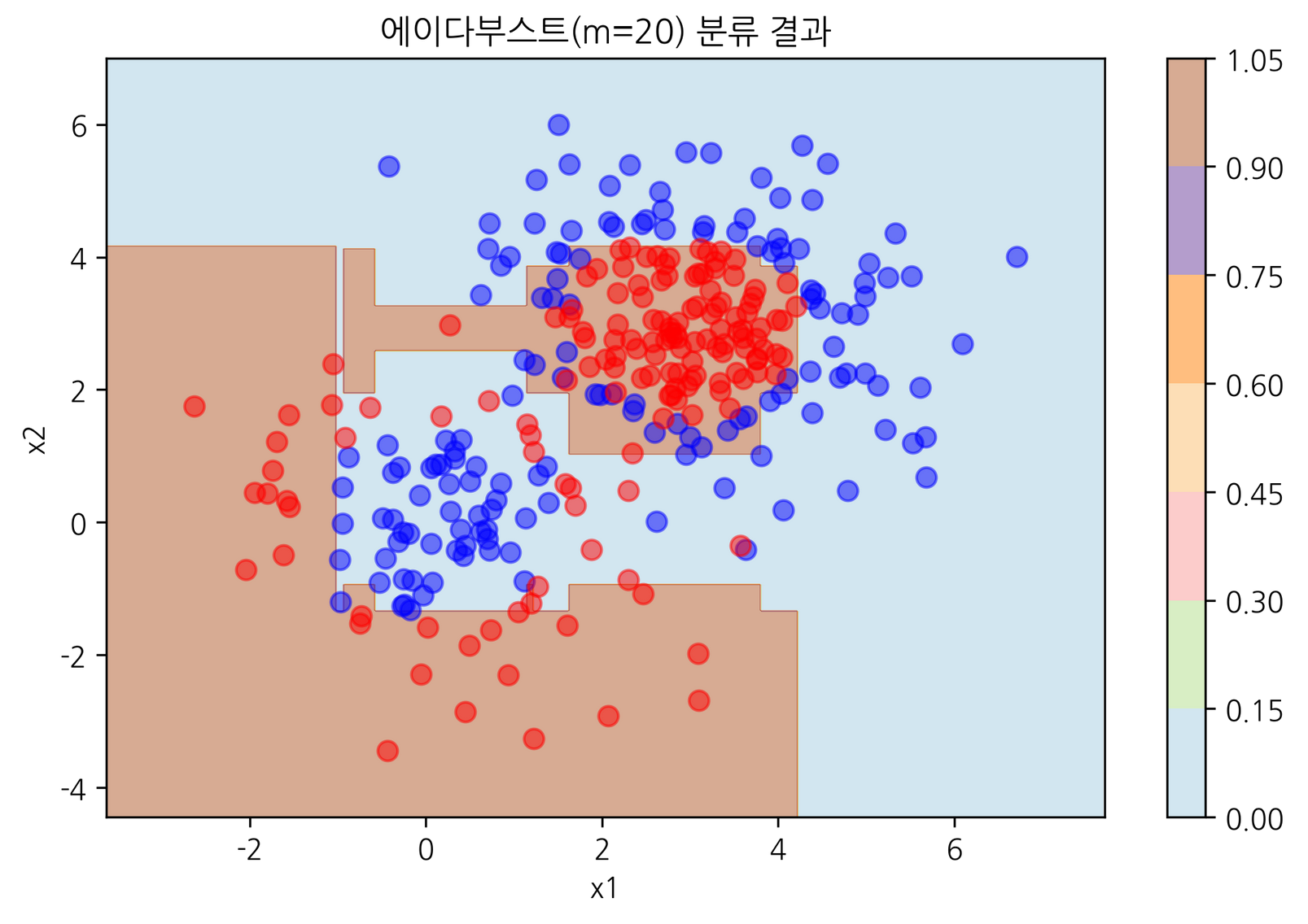
# 분류 결과 출력
plot_result(model_ada, "에이다부스트(m=20) 분류 결과")
i 번째 모델집합 분류결과 반영한, 데이터포인트 별 가중치 시각화 - 1
막대 그래프 사용해서 시각화 했다.
1
2
3
4
5
6
7
8
9
10
11
for i in range(1, 21) :
    plt.subplot(4,5,i)

    xx = model_ada.sample_weight[i-1] # i 번째 모델 집합 분류결과 반영한 데이터포인트 별 가중치
    plt.bar(range(len(xx)), xx)
    plt.title(f'{i}')
    plt.axis('off')

plt.suptitle('300개 데이터 별 가중치 변화')
plt.tight_layout()
plt.show()

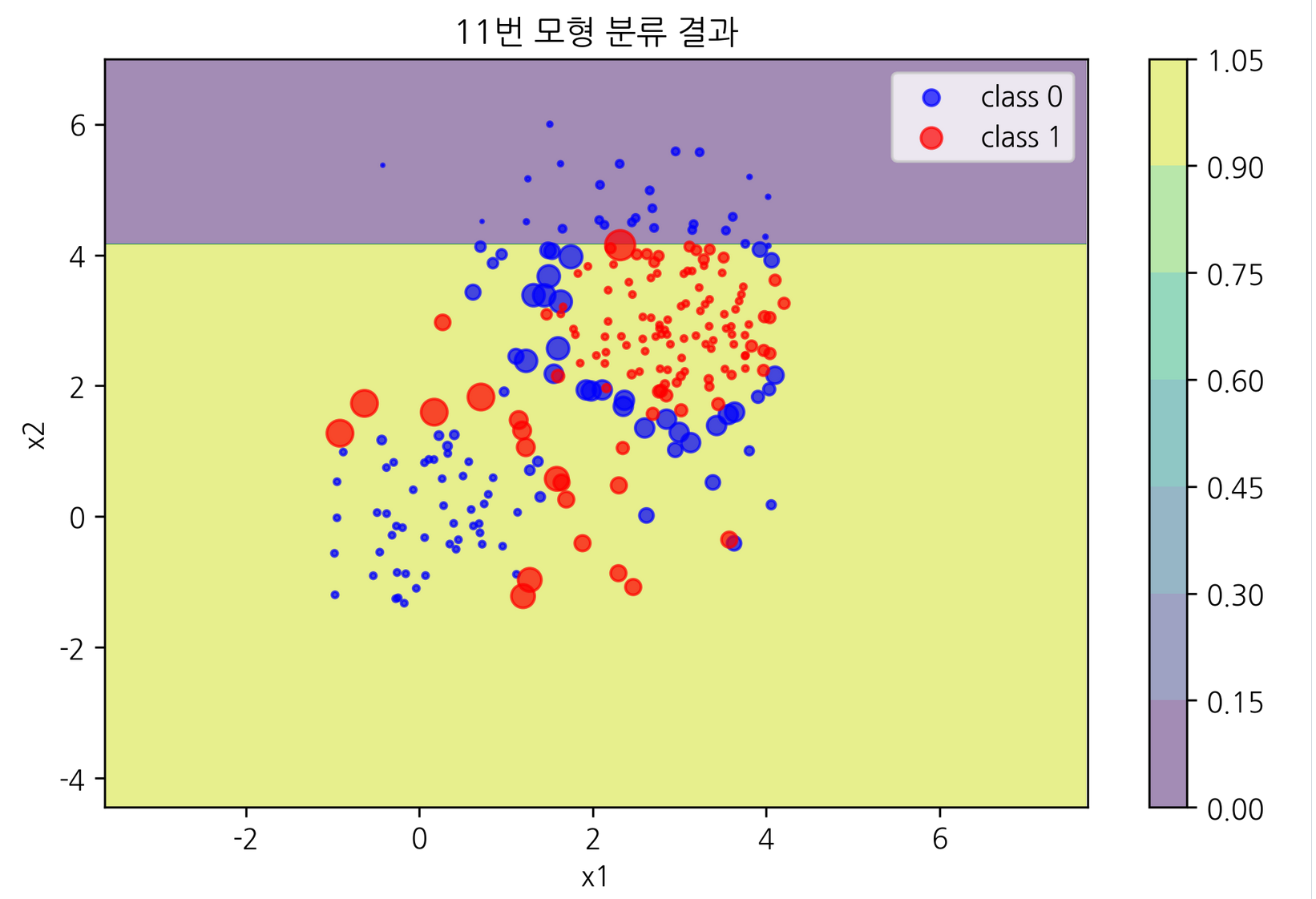
i 번째 모델집합 분류결과 반영한, 데이터포인트 별 가중치 시각화 - 2
스캐터플롯 사용해서 시각화 했다.
가중치 크면(모델들이 자주 틀린 데이터포인트면) 점 크기 크고,
모델들이 잘 맞춘 데이터포인트면 점 크기 작다.
1
2
3
4
5
6
7
8
9
10
11
12
13
14
15
16
17
18
19
20
21
22
23
24
25
26
27
28
29
30
def plot_result2(model, legend=False, s=50, title='분류결과') :
    x1_min, x1_max = X[:,0].min() - 1 , X[:,0].max() + 1 # 입력행렬 X의 X 축 최솟값 & 최댓값
    x2_min, x2_max = X[:,1].min() - 1, X[:, 1].max() + 1 # 입력행렬 X 의 Y 축 최솟값 & 최댓값

    # x 축 최소 최대, y축 최소 최대 이용해서 정사각형 좌표 생성
    xx1, xx2 = np.meshgrid(np.arange(x1_min, x1_max, 0.02), np.arange(x2_min, x2_max, 0.02))  # xx1 = 정사각형 x 좌표, xx2 = 정사각형 y 좌표

    # 정사각형 2차원 평면 위 각 점에 대한 모델의 예측 결과: Y. 1 또는 0이다.
    Y = model.predict(np.c_[xx1.ravel(), xx2.ravel()]).reshape(xx1.shape)

    # 정사각형 각 위 점에 예측 결과 Y 결합; 3차원 그래프 2차원 평면에 색깔로 표현.
    cs = plt.contourf(xx1, xx2, Y, alpha=0.5)

    # 맨 처음 표본 데이터 그래프에 함께 표현
    for i, n, c in zip(range(2), '01', 'br') :
        idx = np.where(y == i) # y 정답값이 i 인 X 행렬 레코드 행.
        plt.scatter(X[idx, 0], X[idx, 1], c=c, s=s[idx], alpha=0.7, label=f'class {i}')

    plt.xlim(x1_min, x1_max)
    plt.ylim(x2_min, x2_max)
    plt.xlabel('x1')
    plt.ylabel('x2')
    plt.title(title)
    plt.colorbar(cs)
    if legend : plt.legend()
    plt.grid(False)
    plt.show()

for i in range(11, 19) :
    plot_result2(model_ada.estimators_[i], legend=True, s=(4000*model_ada.sample_weight[i-1]).astype(int), title=f'{i}번 모형 분류 결과')
결과 이미지는 11번 모형과 18번 모형 둘 만 기록했다.

학습률과 과적합
에이다부스트 모델 집합에 약 분류기 계속 추가 할 수록, 모델은 훈련 데이터에 과적합 되는 경향이 있다.
잘 틀리는 데이터 가장 잘 맞추는 약 분류기(개별모형) 계속 모델 집합에 추가하다 보니 나타나는 현상이다.
에이다부스트 모델 과적합 억제하려면, 학습률(learning rate) 을 1 미만으로 적절히 낮추면 된다.
학습률에 따라 학습/검증 상황이 어떻게 달라지는 지 보자.
1
2
3
4
5
6
7
8
9
10
11
12
13
14
15
16
17
18
learning_list = np.arange(0.001, 0.011, 0.001)

ind = 1
for i in learning_list :
    train_acc = []
    test_acc = []

    for n in range(1, 1101, 100) :
        model = AdaBoostClassifier(DecisionTreeClassifier(max_depth=1), n_estimators=n, learning_rate=i).fit(x_train, y_train)

        train_acc.append(accuracy_score(y_train, model.predict(x_train)))
        test_acc.append(cross_val_score(model, x_test, y_test, cv=5).mean())

    plt.subplot(2,5,ind)
    plt.plot(range(len(range(1, 1101, 100))), train_acc)
    plt.plot(range(len(range(1, 1101, 100))), test_acc)
    ind += 1
plt.tight_layout()

위 그래프 10개는 학습률을 0.001 부터 0.01 까지 10개 줬을 때, 각각 약 분류기 갯수 1에서 100까지 늘려가며 학습 정확도 / 검증 교차검증 정확도 평균 을 그래프로 시각화 한 것이다.
한편 아래 경우는 ‘개별 모델 갯수 증가할 때, 학습률 높으면 과적합이 잘 발생한다’를 위 경우보다 더 분명하게 보여준다.

빨간색이 테스트셋에서 검증 성능, 파란색이 훈련셋에서 성능 나타낸다. 학습률이 0.8 일 때 까지는 과적합 나타나지 않다가, 0.9가 되면서 과적합이 나타났다.
그래디언트 부스트(Gradient Boost)
정의
최적화 알고리즘 중 최급강하법(Gradient Descent) 이용해, 끊임없이 손실 줄이며 모델 업데이트 하는 알고리즘.
최급강하법 알고리즘
정의:
시작위치에서 손실 가장 크게 감소하는 방향(손실함수 기울기 가장 가파르게 감소하는 방향) 으로 계속 이동하며, 손실함수 최소점 찾는 알고리즘.
손실함수 위 점과 점 이동:
$x_{m+1} = x_{m} - \mu\frac{df}{dx}$
다음 위치 $x_{m+1}$ : 시작점 $x_{m}$ 에서의 그레디언트 벡터 반대 방향으로, 스텝사이즈 $\mu$ 만큼 이동한 위치
- 다음 위치 $x_{m+1}$ 은 $x_{m}$ 보다 손실 감소한 위치다.
위 식을 변형하면 아래와 같다.
$\Rightarrow x_{m+1} = x_{m} + \mu(-\frac{df(x_{m})}{dx})$
$x_{m}$ 은 벡터다.
$-\frac{df(x_{m})}{dx}$ 은 벡터 $x_{m}$ 의 그레디언트 벡터에 - 를 취한 것이다. 곧, 그레디언트 벡터 방향 정 반대로 바꾼 것이다.
$-\frac{df(x_{m})}{dx}$ 에 스텝사이즈 $\mu$ 곱하면 negative gradient 의 길이가 조정된다.
벡터 $x_{m}$ 에 $\mu(-\frac{df(x_{m})}{dx})$ 를 더한 위치가 손실 감소한 다음 위치 $x_{m+1}$ 이다.
*벡터 $x_{m}$ 에 $\mu(-\frac{df(x_{m})}{dx})$ 를 더한 결과는 시점이 $x_{m}$ 이고 화살표 끝 점이 $x_{m+1}$ 인 벡터와도 같다.
그래디언트 부스팅은 위 최급강하법 알고리즘을 모델 업데이트에 적용한 앙상블 알고리즘이다.
모델 업데이트 방법
$c_{m} = c_{m-1} -\alpha_{m}\frac{\partial{L(y, c_{m-1})}}{\partial{c_{m-1}}}$
$\Rightarrow c_{m} = c_{m-1} +\alpha_{m}(-\frac{\partial{L(y, c_{m-1})}}{\partial{c_{m-1}}})$
- $c_{m}$ : 새 모델(손실함수 위 새 위치)
- $c_{m-1}$ : 기존 모델(손실함수 위 기존 위치)
- $\alpha_{m}$ : 스텝사이즈(이동거리)
- $-\frac{\partial{L(y, c_{m-1})}}{\partial{c_{m-1}}}$: negative gradient. 방향 정 반대로 바꾼, 점 $c_{m-1}$ 에서의 그레디언트 벡터. $c_{m-1}$ 이 이동해야 할 방향이다.
모델 $c_{m}, c_{m-1}$ 을 손실함수 위 점(벡터)로 생각하면 된다.
위 식의 의미를 해석하면, ‘기존 모델 $c_{m-1}$ 보다 손실 감소하는 방향과 거리에 위치한 새 모델 $c_{m}$ 을 찾은 것’ 이다.
그래디언트 부스팅 알고리즘은 위 식 계산을 반복적으로 수행하며, 계속 손실 줄이는 방식으로 모델 반복적 업데이트 한다.
전체 알고리즘 진행 과정
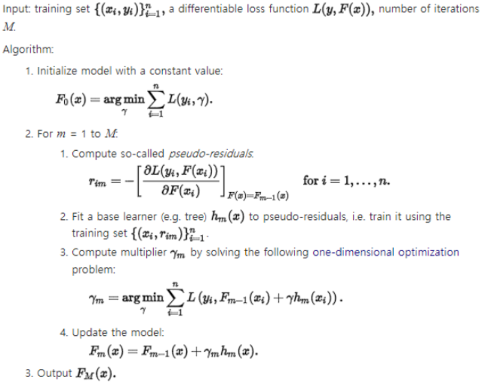
[ 이미지 출처: https://m.blog.naver.com/winddori2002/221837065744?view=img_2 ]
- 특성변수들과 타겟값으로 이루어진 훈련용 데이터셋 준비, 모델 업데이트 할 총 횟수 $M$ 지정, 그리고 미분가능한 손실함수 $L(y, f(x))$를 정의한다.
- 손실함수 위 첫 시작위치로, $F_{0}(x) = argmin_{r}{(\sum_{i=1}^{n}{L(y_{i}, r)})}$ 를 만족하는 상수 $r$ 을 찾는다. 예컨대 만약 손실함수 $L$ 이 오차 제곱 이라면, 훈련 데이터셋 타겟값 $y_{i}$ 와 오차 제곱합 최소로 만드는 상수 $r$ 을 찾고, 최적화 시작점으로 삼는다. $(F_{0}{(x)} = r)$
- 최적화 시작점 $r$ 에서의 negative gradient 벡터를 찾는다. 타겟값 $y_{i} (i=1,…,n)$ 별로 서로 다른 negative gradient $n$ 개 생성된다. $r_{im} = negative$ $gradient_{1…n}$
- 앙상블 약 분류기인, 임의의 의사결정회귀나무 $h_{m}(x)$ 를 3에서 구한 negative gradient 들을 타겟값으로 삼아 훈련시킨다. 즉, 1의 훈련용 데이터셋에서 $x$ 특성변수들은 그대로 두고, $y$ 타겟값만 negative gradient 들로 바꾼 뒤 $h_{m}(x)$ 모델에 넣어 훈련시킨다. 모델이 학습하는 것은 긱 데이터포인트에 대해, ‘손실 최소화 하기 위한 손실함수 위 이동 방향’ 이다. 이제 $h_{m}(x)$ 모델은 임의의 새로운 입력 $x$ 를 받게 되면 $x$ 에 대응되는 negative gradient 예측값을 내놓을 것이다. 즉, ‘현재모델 $F_{m-1}(x)$ 기준, 모델 손실 최소화 할 수 있는 방향 예측치’를 출력할 것이다.
- $r_{m} = argmin_{r_{m}}{\sum_{i=1}^{n}(y_{i} - F_{m-1}(x_{i}) + r_{m} h_{m}(x_{i}))^{2}}$ 만족하는 스텝사이즈 $r_{m}$ 찾는다.
- 기존모델 $F_{m-1}(x) +$ 스텝사이즈 $r_{m}$ $\times$ negative gradient 예측치 출력하는 약 분류기 $h_{m}(x)$ $=$ 업데이트 된 모델 $F_{m}(x)$
- 위 3번에서 6번 과정을 $M$ 번 반복한다. 손실을 계속 줄여가면서, 모델이 계속 업데이트 된다.
그래디언트 부스트 기반 알고리즘 종류
- XGBoost
- LightGBM
구현
1
2
3
4
5
# 사이킷런 그래디언트 부스트 분류기 호출
from sklearn.ensemble import GradientBoostingClassifier # 내부 약 분류기로 의사결정회귀나무 사용

# 분류 모델 준비
model_grad = GradientBoostingClassifier(n_estimators=100, max_depth=2, random_state=0) # {약 분류기 갯수: 100개, 약 분류기 깊이: 2, 랜덤시드:0}
샘플 데이터셋 구성
1
2
3
4
5
6
7
8
9
10
11
12
13
14
15
16
17
18
19
20
%%time
%matplotlib inline

# 데이터셋 호출
from sklearn.datasets import make_gaussian_quantiles

# 임의 생성 데이터셋
x1, y1 = make_gaussian_quantiles(cov=2.0, random_state=0, n_samples=200, n_features=2, n_classes=2, shuffle=True)
x2, y2 = make_gaussian_quantiles(cov=2.0, random_state=1, n_samples=200, n_features=2, n_classes=2, shuffle=True)

X = np.concatenate([x1, x2], axis=0) ; y = np.concatenate([y1, y2], axis=0)

idx_0 = np.where(y==0); idx_1 = np.where(y==1)

# 데이터셋 시각화
plt.scatter(X[idx_0, 0], X[idx_0,1], c='r', label='class=0')
plt.scatter(X[idx_1, 0], X[idx_1,1], c='g', label='class=1')
plt.legend()
plt.title('Sample Data')
plt.show()

이렇게 생긴 데이터셋이다.
1
2
3
4
5
6
7
8
9
10
11
# 모델 성능 검증에 쓸 데이터셋 형태 둘러보기
x1_min, x1_max = x1[:,0].min(), x1[:,0].max()
x2_min, x2_max = x2[:,0].min(), x2[:,0].max()

xx1, xx2 = np.meshgrid(np.arange(x1_min, x1_max, 1), np.arange(x2_min, x2_max, 1))
plt.scatter(xx1, xx2)
plt.axis('off')
plt.show()

xx1, xx2 = np.meshgrid(np.arange(x1_min, x1_max, 0.02), np.arange(x2_min, x2_max, 0.02))
plt.scatter(xx1, xx2)

그래디언트 부스트 분류기에 훈련용 데이터 학습시키기
1
2
3
4
%%time

# 그래디언트부스트 분류기, 훈련용 데이터 학습
fitted_model = model_grad.fit(X, y)
그래디언트 부스트 분류기로 새 데이터셋의 정답 예측
1
2
3
4
5
6
7
8
9
10
11
12
13
14
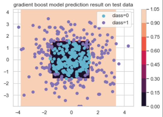
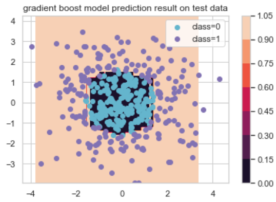
# 그래디언트부스트 분류기, 새 데이터셋 예측
xx_predict = np.c_[xx1.ravel(), xx2.ravel()]
Y = fitted_model.predict(xx_predict).reshape(xx1.shape)
# 새 데이터셋 예측 결과 시각화
cs = plt.contourf(xx1, xx2, Y)
plt.colorbar(cs)
idx_0 = np.where(y==0); idx_1 = np.where(y==1)
plt.scatter(X[idx_0, 0], X[idx_0,1], c='c', label='class=0')
plt.scatter(X[idx_1, 0], X[idx_1,1], c='m', label='class=1')
plt.legend()
plt.title('gradient boost model prediction result on test data')
plt.show()

손실 계속 줄여가며 모델 업데이트하는 그래디언트부스트 모델이 상당히 정확하게 예측해냈음을 확인할 수 있었다.
개별 약 분류기 분류 결과 시각화; 1번째 약 분류기(의사결정회귀나무)
1
2
3
4
5
6
7
8
9
10
11
12
13
14
15
16
17
18
19
20
21
22
23
24
25
print(f'앙상블 weak learner 갯수: {len(fitted_model.estimators_)}')
print(fitted_model.estimators_[0][0]) # 약 분류기는 모두 의사결정회귀나무다.

# 시각화 함수 정의
def plot_result(model,x1, x2, X, y) :
    x1_min, x1_max = x1[:,0].min(), x1[:,0].max()
    x2_min, x2_max = x2[:,0].min(), x2[:,0].max()
    xx1, xx2 = np.meshgrid(np.arange(x1_min, x1_max, 0.02), np.arange(x2_min, x2_max, 0.02))

    fitted_model = model.fit(X, y)
    xx_predict = np.c_[xx1.ravel(), xx2.ravel()]
    Y = fitted_model.predict(xx_predict).reshape(xx1.shape)

    cs = plt.contourf(xx1, xx2, Y)
    plt.colorbar(cs)

    idx_0 = np.where(y==0); idx_1 = np.where(y==1)
    plt.scatter(X[idx_0, 0], X[idx_0,1], c='c', label='class=0')
    plt.scatter(X[idx_1, 0], X[idx_1,1], c='m', label='class=1')
    plt.legend()
    plt.title('gradient boost model prediction result on test data')
    plt.show()

# 첫번째 개별 분류기 분류결과
plot_result(fitted_model.estimators_[0][0],x1,x2, X, y)

에이다부스트 모델 분류 결과와 비교
1
2
3
4
5
6
7
8
9
# 에이다부스트모델 결과와 비교
from sklearn.ensemble import AdaBoostClassifier
from sklearn.tree import DecisionTreeClassifier

# 에이다부스트 모델
adamodel = AdaBoostClassifier(DecisionTreeClassifier(max_depth=1), n_estimators=100)
fitted_ada = adamodel.fit(X, y)

plot_result(adamodel, x1, x2, X, y)
XGBoost 알고리즘
정의
모든 작업을 병렬처리하는, 그래디언트 부스트 알고리즘.
효용
- 과적합에 robust 하다.
- 성능과 효율 모두 뛰어나다.
구현
1
2
3
4
5
6
7
%%time # 작업수행시간 측정
import xgboost

# xgboost 모델 정의
model_xgb = xgboost.XGBClassifier(n_estimators=100, max_depth=1, random_state=0)

model_xgb.fit(X,y)
CPU times: total: 266 ms
Wall time: 83.7 ms
XGBoost 분류기; 설정 가능한 하이퍼파라미터들
XGBClassifier(base_score=0.5, booster=’gbtree’, callbacks=None, colsample_bylevel=1, colsample_bynode=1, colsample_bytree=1, early_stopping_rounds=None, enable_categorical=False, eval_metric=None, gamma=0, gpu_id=-1, grow_policy=’depthwise’, importance_type=None, interaction_constraints=’’, learning_rate=0.300000012, max_bin=256, max_cat_to_onehot=4, max_delta_step=0, max_depth=1, max_leaves=0, min_child_weight=1, missing=nan, monotone_constraints=’()’, n_estimators=100, n_jobs=0, num_parallel_tree=1, predictor=’auto’, random_state=0, reg_alpha=0, reg_lambda=1, …)
새 데이터셋에 대한 분류 결과 시각화
1
2
# 새 데이터셋 분류 결과 시각화
plot_result(model_xgb, x1, x2, X, y)

LightGBM 알고리즘
XGBoost 알고리즘과 마찬가지로, 그래디언트 부스트 알고리즘을 기반으로 한다.
효용
- 속도가 빠르다 (GB > XGBoost > LightGBM)
단점
- 데이터셋 갯수가 10,000 개 이하일 때는 과적합에 빠지기 쉽다. 따라서 갯수가 10,000개 초과하는 데이터셋에 사용하는 것이 좋다.
구현
1
2
3
4
5
6
7
8
9
10
11
%%time
import lightgbm

# lightgbm 모델 정의
model_lgbm = lightgbm.LGBMClassifier(n_estimators=100, max_depth=1, random_state=0)

# 모델 학습
model_lgbm.fit(X, y)

# 결과 시각화
plot_result(model_lgbm, x1, x2, X, y)