
‘프로그래머가 알아야 할 알고리즘 40’(임란 아마드 지음, 길벗 출판사) 을 통해 로지스틱 회귀, 서포트벡터 머신, 나이브 베이즈 알고리듬을 공부하고 나서, 그 내용을 내 언어로 바꾸어 기록한다.
로지스틱 회귀(Logistic Regression) 분류 알고리즘
이진분류에 로지스틱 함수(시그모이드 함수) 사용하는, 이진분류 알고리즘이다.
목표
모델 손실 최소화 하는, 최적의 $W$, $j$ 찾기.
사용조건
- 모든 특성변수는 서로 독립이어야 한다.
예측값 계산
$\hat{y} = \sigma{(wX + j)}$
- $\hat{y}$ 는 타겟 $y$ 예측값
- $X$ 가 입력 데이터셋
- $w$ 는 가중치
- $\sigma{()}$ 는 로지스틱(시그모이드) 함수
로지스틱 함수
$\sigma{(x)} = \frac{1}{1 + e^{-x}}$
1
2
3
4
5
6
7
8
9
10
11
12
import numpy as np
def logistic(x) :
    return 1/(1+np.e**(-x))
xx = np.linspace(-6, 6, 100000)
yy = logistic(xx)

plt.plot(xx, yy)
plt.title('Logistic(Sigmoid) function')
plt.axhline(0.5, c='r', ls='--')
plt.axhline(1, c='g')
plt.axhline(0, c='g')
plt.show()
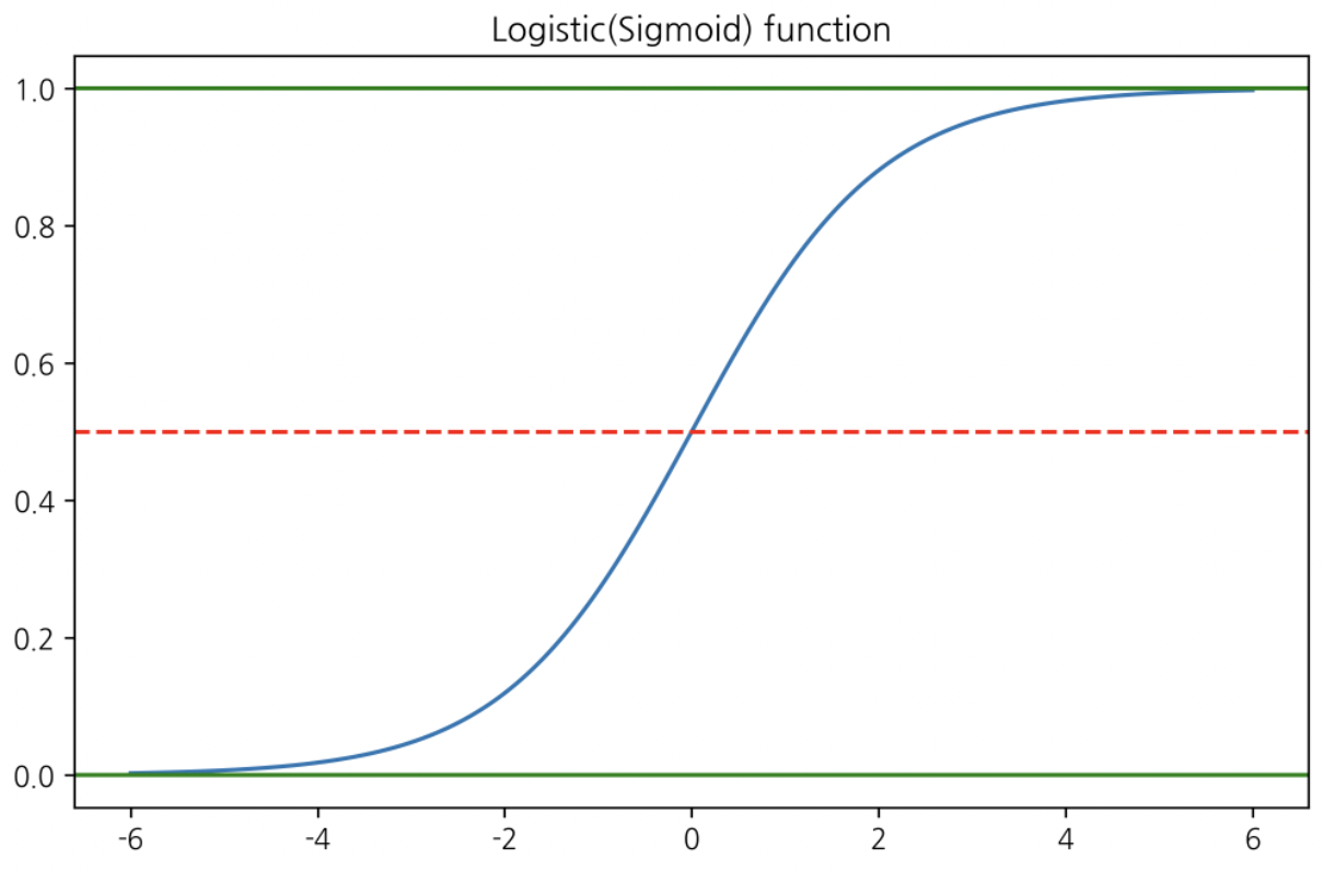
$wX + j$ 값을 계산 후 로지스틱 함수 $\sigma$ 에 넣는다.
그러면 위와 같은 형상이 생성된다.
1개 데이터레코드의 결과값이 0.5 를 넘으면 1, 0.5보다 낮으면 0으로 이진분류 한다.
개별 데이터레코드에 대한 손실함수
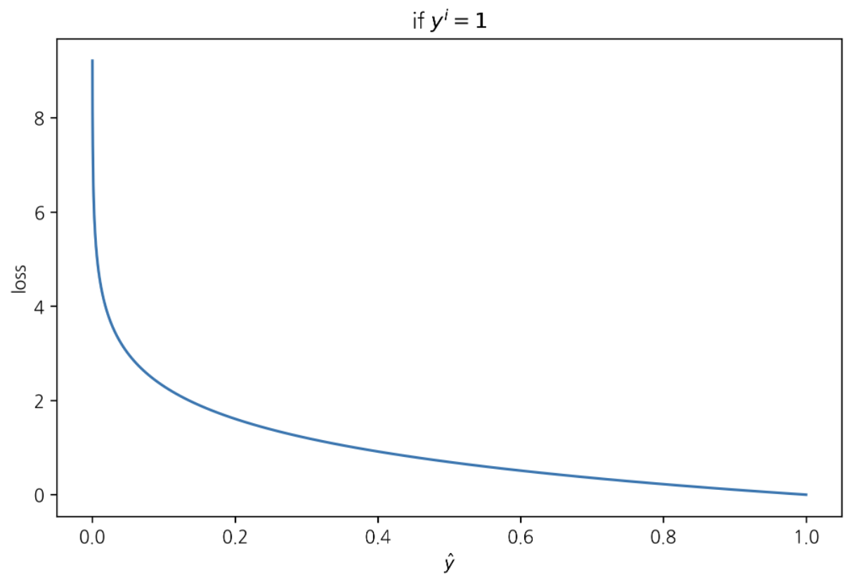
$loss = -(y^{i}\log{\hat{y}^{i}} + (1-y^{i})\log{(1-\hat{y}^{i})})$
if $y^{i} = 1$ $\Rightarrow$ $loss = -\log{\hat{y}^{i}}$
이 경우 손실이 최소화 되려면 $\hat{y}^{i}$ 가 최대화 되어야 한다(1쪽으로 가야한다)
1
2
3
4
5
6
7
8
9
10
xx = np.linspace(0, 1, 10000)

def loss1(y) :
    return -np.log(y)
yy = loss1(xx)
plt.plot(xx, yy)
plt.xlabel('$\hat{y}$')
plt.ylabel('loss')
plt.title('if $y^{i} = 1$')
plt.show()
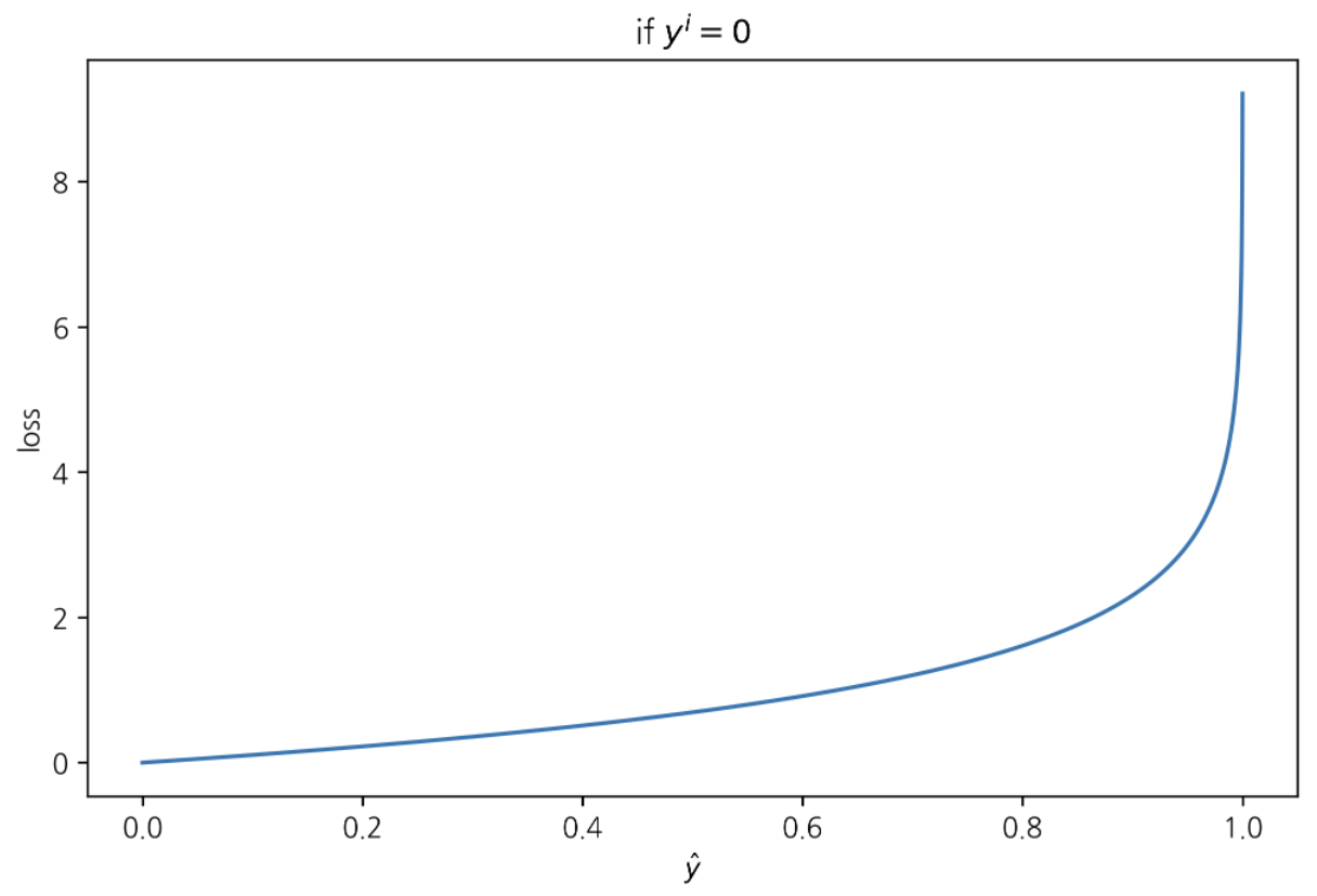
if $y^{i} = 0 \Rightarrow loss = -\log{(1-\hat{y}^{i})}$
이 경우 손실이 최소화 되려면 $\hat{y}^{i}$ 가 최소화 되어야 한다(0쪽으로 가야한다)
1
2
3
4
5
6
7
8
9
xx = np.linspace(0, 1, 10000)
def loss2(y) :
    return -np.log(1-y)
yy = loss2(xx)
plt.plot(xx, yy)
plt.xlabel('$\hat{y}$')
plt.ylabel('loss')
plt.title('if $y^{i} = 0$')
plt.show()
로지스틱 회귀 한게
로지스틱 회귀모델은 입력 데이터가 복잡해질 수록 성능 떨어지는 경향, 있다.
로지스틱 회귀는 단순한 패턴 분석 및 분류할 때 괜찮은 성능 기록한다.
로지스틱 회귀모델로 붓꽃 이진분류 하기
1
2
3
4
5
6
7
8
9
10
11
12
13
14
15
16
17
18
19
20
21
22
23
24
25
26
27
28
29
30
31
32
33
34
%matplotlib inline

# 로지스틱 회귀모형 이용한 이진분류
from sklearn.datasets import load_iris
from sklearn.model_selection import train_test_split
from sklearn.metrics import confusion_matrix
from sklearn.metrics import accuracy_score

data = load_iris()
X = data.data
y = data.target

idx0 = np.where(y==0)
idx1 = np.where(y==1)
idx = np.concatenate([idx0, idx1], axis=1)

# 특성변수들
X = X[idx, :]
# 레이블
y = y[idx]

# 훈련용 셋과 테스트용 셋으로 입력 데이터셋 분리
x_train, x_test, y_train, y_test = train_test_split(X[0], y[0], test_size=0.25)

# 로지스틱 회귀모형 정의
from sklearn.linear_model import LogisticRegression
classifier = LogisticRegression(random_state=0) # random_state=0 ; 모형에 데이터 투입할 때 Shuffle 하기 위해서 지정
classifier.fit(x_train, y_train) # 훈련 데이터에 대해 학습

# 테스트 데이터 예측
y_pred = classifier.predict(x_test)

# 혼동행렬 출력; 모델이 레이블 잘 맞췄는지 확인
cm = confusion_matrix(y_test, y_pred) ; cm
array([[16, 0], [ 0, 9]], dtype=int64)
1
accuracy_score(y_test, y_pred)
1.0
로지스틱 회귀모델로 임의 생성 데이터셋 이진분류 하기
1
2
3
4
5
6
7
8
9
10
11
12
13
14
15
16
17
18
# 데이터셋 호출
from sklearn.datasets import make_gaussian_quantiles
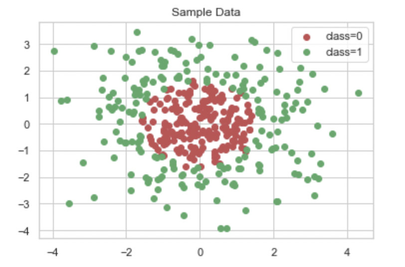
# 임의 생성 데이터셋
x1, y1 = make_gaussian_quantiles(cov=2.0, random_state=0, n_samples=200, n_features=2, n_classes=2, shuffle=True)
x2, y2 = make_gaussian_quantiles(cov=2.0, random_state=1, n_samples=200, n_features=2, n_classes=2, shuffle=True)
# X: 입력 데이터셋 , y: 타겟
X = np.concatenate([x1, x2], axis=0) ; y = np.concatenate([y1, y2], axis=0)
idx_0 = np.where(y==0); idx_1 = np.where(y==1)
# 데이터셋 시각화
plt.scatter(X[idx_0, 0], X[idx_0,1], c='r', label='class=0')
plt.scatter(X[idx_1, 0], X[idx_1,1], c='g', label='class=1')
plt.legend()
plt.title('Sample Data')
plt.show()
모델 성능 검증에 쓸 데이터셋 생성
1
2
3
4
5
6
7
8
9
10
11
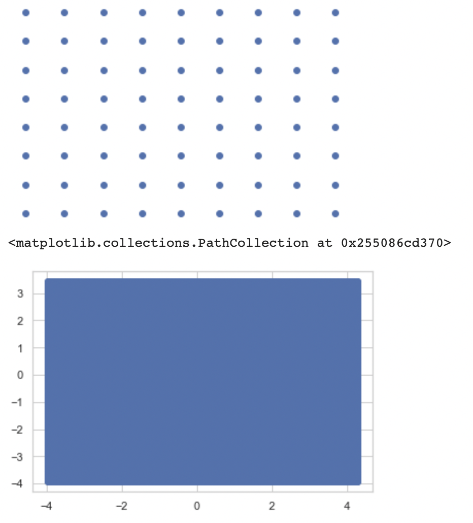
# 모델 성능 검증에 쓸 데이터셋 형태 둘러보기
x1_min, x1_max = X[:,0].min(), X[:,0].max()
x2_min, x2_max = X[:,1].min(), X[:,1].max()
xx1, xx2 = np.meshgrid(np.arange(x1_min, x1_max, 1), np.arange(x2_min, x2_max, 1))
plt.scatter(xx1, xx2)
plt.axis('off')
plt.show()
xx1, xx2 = np.meshgrid(np.arange(x1_min, x1_max, 0.02), np.arange(x2_min, x2_max, 0.02))
plt.scatter(xx1, xx2)
1
2
3
4
5
6
7
8
9
10
11
12
13
14
15
16
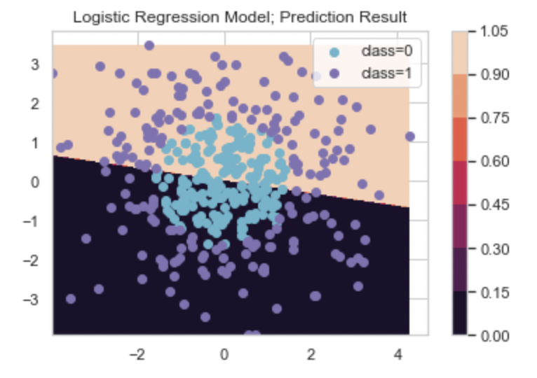
# 로지스틱 회귀 분류기 학습
classifier.fit(X, y)
# 로지스틱 회귀 분류기 새 데이터 예측
xx_predict = np.c_[xx1.ravel(), xx2.ravel()]
Y = classifier.predict(xx_predict).reshape(xx1.shape)
# 예측 결과 시각화
cs = plt.contourf(xx1, xx2, Y)
plt.colorbar(cs)
idx_0 = np.where(y==0); idx_1 = np.where(y==1)
plt.scatter(X[idx_0, 0], X[idx_0,1], c='c', label='class=0')
plt.scatter(X[idx_1, 0], X[idx_1,1], c='m', label='class=1')
plt.legend()
plt.title('Logistic Regression Model; Prediction Result')
plt.show()
로지스틱 회귀모델로 이진분류 한 결과, XGBoost(그래디언트 부스트) 모델 결과와 비교하기
1
2
3
4
5
6
# xgboost 모델 정의 후 학습
import xgboost

xgb_model = xgboost.XGBClassifier(n_estimators=100, max_depth=1, random_state=0)

xgb_model.fit(X, y)
XGBClassifier(base_score=0.5, booster=’gbtree’, callbacks=None, colsample_bylevel=1, colsample_bynode=1, colsample_bytree=1, early_stopping_rounds=None, enable_categorical=False, eval_metric=None, gamma=0, gpu_id=-1, grow_policy=’depthwise’, importance_type=None, interaction_constraints=’’, learning_rate=0.300000012, max_bin=256, max_cat_to_onehot=4, max_delta_step=0, max_depth=1, max_leaves=0, min_child_weight=1, missing=nan, monotone_constraints=’()’, n_estimators=100, n_jobs=0, num_parallel_tree=1, predictor=’auto’, random_state=0, reg_alpha=0, reg_lambda=1, …)
1
2
3
4
5
6
7
8
9
10
11
12
# xgboost 모델 예측
xgb_Y = xgb_model.predict(xx_predict).reshape(xx1.shape)

# 예측 결과 시각화
cs = plt.contourf(xx1, xx2, xgb_Y)
plt.colorbar(cs)
idx_0 = np.where(y==0); idx_1 = np.where(y==1)
plt.scatter(X[idx_0, 0], X[idx_0,1], c='c', label='class=0')
plt.scatter(X[idx_1, 0], X[idx_1,1], c='m', label='class=1')
plt.legend()
plt.title('XGBoost model; prediction result')
plt.show()
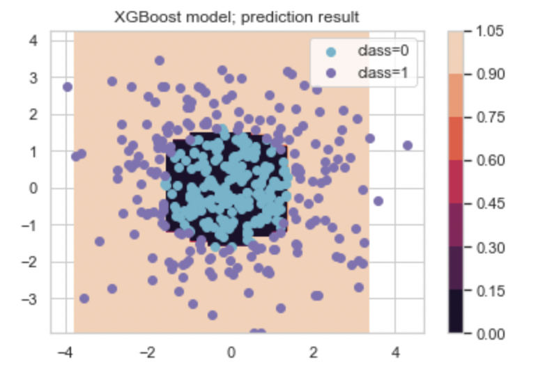
이 경우, 로지스틱 회귀모형은 xgboost 모형보다 분류 정확성이 떨어졌다.
로지스틱 회귀모형으로 분류문제 해결하기 - 2
날씨 예측하기
1
2
3
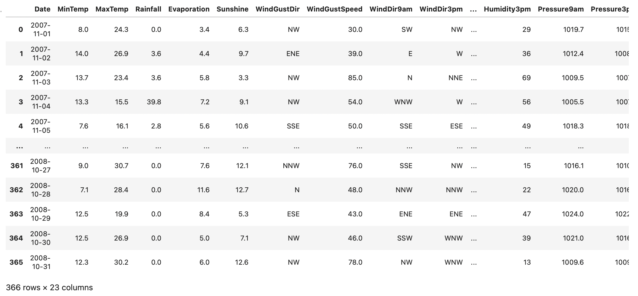
# 데이터셋 로드
df = pd.read_csv('/Users/kibeomkim/Desktop/weather.csv')
df
1
2
3
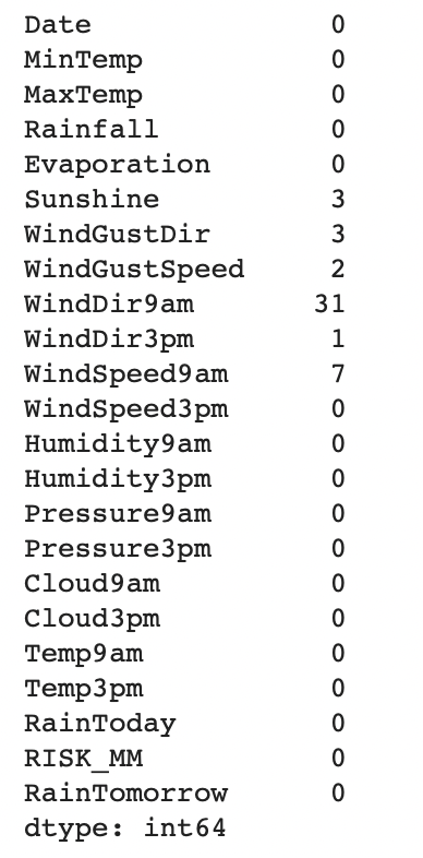
df.info()
df.describe()
df.isnull().sum()
1
2
3
4
5
6
7
8
9
10
11
12
13
14
15
16
17
18
19
mean = df['WindGustSpeed'].mean()
df['WindGustSpeed'] = df['WindGustSpeed'].fillna(mean)
mean = df['Sunshine'].mean()
df['Sunshine'] = df['Sunshine'].fillna(mean)
df['WindSpeed9am'] = df[['WindGustDir', 'WindDir9am', 'WindDir3pm', 'WindSpeed9am']].iloc[:,3].fillna(df['WindSpeed9am'].mean())
df.drop('Date', axis=1, inplace=True)
y = df['RainTomorrow'].values
y_idx = np.where(y=='Yes')
n_idx = np.where(y=='No')
y[y_idx] = 1 ; y[n_idx] = 0
df.drop('RainTomorrow', axis=1, inplace=True)
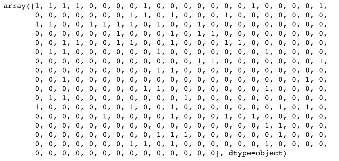
# 타겟
y # 이 값들 타겟으로 잡으면 이진분류 문제가 된다.
1
2
3
4
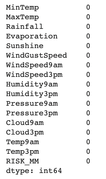
# 5, 7, 8, 19; string 값 가진 특성변수 제외
new_df = df.drop(['WindGustDir', 'WindDir9am', 'WindDir3pm', 'RainToday'], axis=1)
new_df.isnull().sum()
1
2
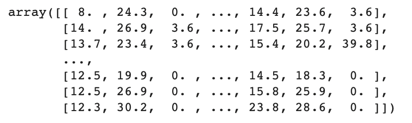
# 입력 특성변수들
X = new_df.values ; X
모델 훈련시키기
1
2
3
4
5
6
7
8
# 훈련용 셋과 테스트용 셋으로 분리
x_train, x_test, y_train, y_test = train_test_split(X, np.array(list(y)), test_size=0.25, random_state=0)

from sklearn.linear_model import LogisticRegression
model = LogisticRegression()

# 모델 훈련시키기
model.fit(x_train, y_train)
모델 성능 확인
1
2
3
4
5
6
7
# 테스트 데이터에 대해 모델 예측
y_pred = model.predict(x_test)

# 정확도 계산 (모델 성능지표 계산)
from sklearn.metrics import accuracy_score
acc_score = accuracy_score(y_test, y_pred)
print(f'로지스틱회귀 이진분류 모델 정확도:{round(acc_score*100, 2)}%')
로지스틱회귀 이진분류 모델 정확도: 97.83%
서포트벡터 머신 (Support Vector Machine) 알고리즘
이진분류 알고리즘이다.
정의
마진 최대화 하는, 초평면 찾기.
- 마진: 초평면과 서포트벡터 사이 거리
- 서포트벡터: 초평면에서 가장 가까운 벡터들을 서포트벡터(support vector) 라고 한다.
$\Rightarrow$ 두 클래스 가장 ‘잘’ 구분하는, 초평면 찾기.
서포트벡터 머신 모형으로 이진분류 문제 해결하기
1
2
3
4
5
6
7
8
9
10
11
12
13
14
15
16
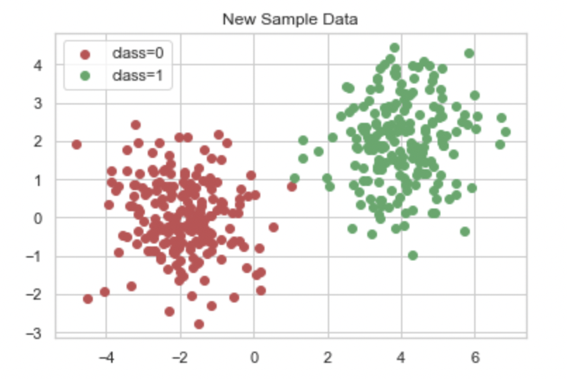
# 임의 데이터셋 생성
x1, y1 = make_gaussian_quantiles(mean=[4,2],cov=1, random_state=3, n_samples=200, n_features=2, n_classes=1, shuffle=True)
x2, y2 = make_gaussian_quantiles(mean=[-2,0],cov=1, random_state=1, n_samples=200, n_features=2, n_classes=1, shuffle=True)
y1 = [1]*len(y1)
# X: 특성변수들, y: 타겟값들
X = np.concatenate([x1, x2], axis=0) ; y = np.concatenate([y1, y2], axis=0)
idx_0 = np.where(y==0); idx_1 = np.where(y==1)
# 생성된 데이터셋 시각화
plt.scatter(X[idx_0, 0], X[idx_0,1], c='r', label='class=0')
plt.scatter(X[idx_1, 0], X[idx_1,1], c='g', label='class=1')
plt.legend()
plt.title('New Sample Data')
plt.show()
1
2
3
4
5
x1_min, x1_max = X[:,0].min(), X[:,0].max()
x2_min, x2_max = X[:,1].min(), X[:,1].max()

xx1, xx2 = np.meshgrid(np.arange(x1_min, x1_max, 0.02), np.arange(x2_min, x2_max, 0.02))
plt.scatter(xx1, xx2)
1
2
3
4
5
6
7
8
9
10
11
12
13
14
15
16
17
18
19
20
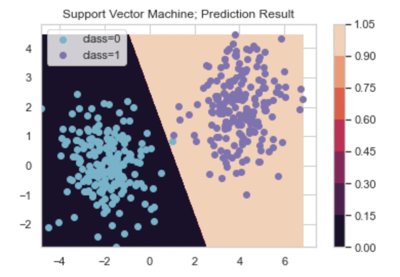
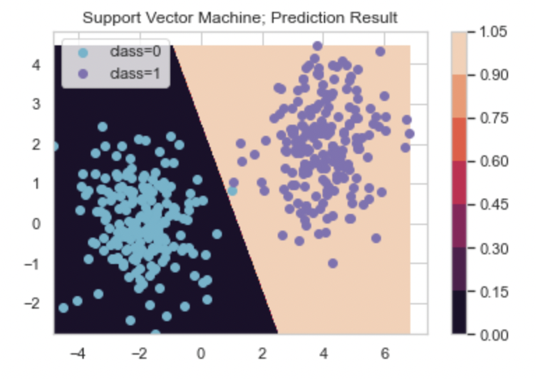
# 서포트벡터 머신
from sklearn.svm import SVC
classifier_svm = SVC(kernel='linear', random_state=0)
# 모델 학습
classifier_svm.fit(X, y)
# 모델 예측
xx_predict = np.c_[xx1.ravel(), xx2.ravel()]
Y = classifier_svm.predict(xx_predict).reshape(xx1.shape)
# 예측 결과 시각화
cs = plt.contourf(xx1, xx2, Y)
plt.colorbar(cs)
idx_0 = np.where(y==0); idx_1 = np.where(y==1)
plt.scatter(X[idx_0, 0], X[idx_0,1], c='c', label='class=0')
plt.scatter(X[idx_1, 0], X[idx_1,1], c='m', label='class=1')
plt.legend()
plt.title('Support Vector Machine; Prediction Result')
plt.show()
나이브 베이즈 알고리즘
확률론 기반 분류 알고리즘.
특징
- 입력 데이터셋 모든 특성변수가 서로 독립 이라는, ‘나이브(naive)’ 한 기본 가정 사용한다.
- 베이즈 정리 사용한다.
나이브 베이즈 모형으로 이진분류 문제 해결하기
1
2
3
4
5
6
7
8
9
10
11
12
13
14
15
16
17
18
19
20
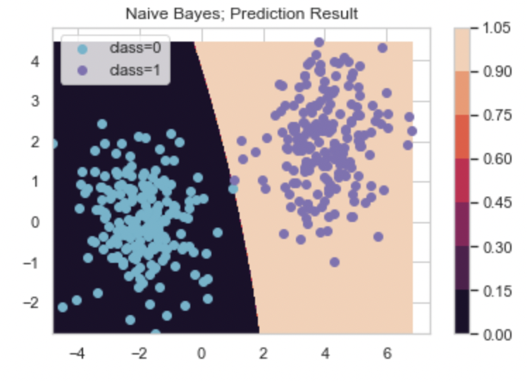
from sklearn.naive_bayes import GaussianNB
# 나이브 베이즈 분류모형
classifier = GaussianNB()
# 모형 학습
classifier.fit(X, y)
# 모형 예측
yy = classifier.predict(xx_predict).reshape(xx1.shape)
# 모형 에측 결과 시각화
cs = plt.contourf(xx1, xx2, yy)
plt.colorbar(cs)
idx_0 = np.where(y==0); idx_1 = np.where(y==1)
plt.scatter(X[idx_0, 0], X[idx_0,1], c='c', label='class=0')
plt.scatter(X[idx_1, 0], X[idx_1,1], c='m', label='class=1')
plt.legend()
plt.title('Naive Bayes; Prediction Result')
plt.show()
분류 알고리즘 별 성능 비교
- 의사결정나무
- xgboost(앙상블-부스트-그래디언트 부스트)
- 랜덤포레스트(앙상블-취합-배깅)
- 로지스틱 회귀
- 서포트벡터 머신
- 나이브 베이즈
같은 분류문제에 대해 위 6개 분류 알고리즘 분류성능을 비교할 것이다.
1
2
3
4
5
6
7
8
9
10
11
12
13
14
15
16
17
18
19
20
# 분류알고리즘 별 성능 비교
from sklearn.tree import DecisionTreeClassifier
import xgboost
from sklearn.ensemble import RandomForestClassifier
from sklearn.linear_model import LogisticRegression
from sklearn.svm import SVC
from sklearn.naive_bayes import GaussianNB
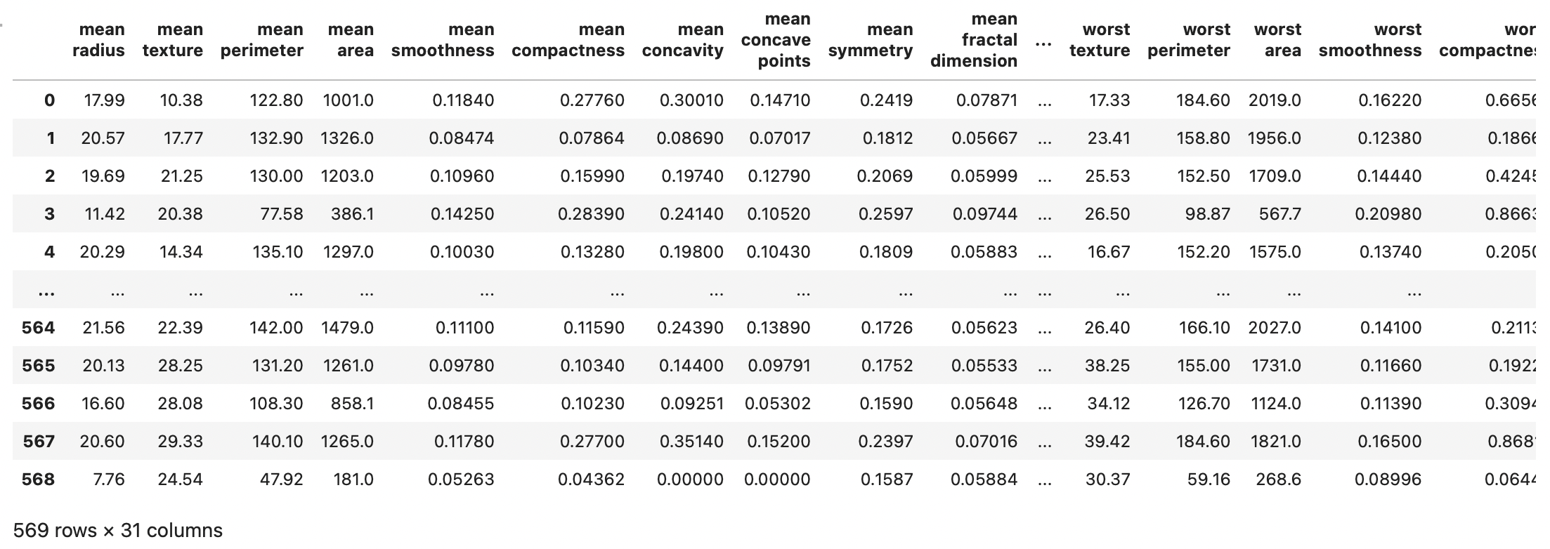
# 유방암 데이터셋 로드
from sklearn.datasets import load_breast_cancer
data = load_breast_cancer()
X = data.data
y = data.target
feature_names = data.feature_names
df = pd.DataFrame(X, columns=feature_names)
df['y'] = y
df
1
df.shape
(569, 31)
1
df.isnull().sum()
mean radius 0
mean texture 0
mean perimeter 0
mean area 0
mean smoothness 0
mean compactness 0
mean concavity 0
mean concave points 0
mean symmetry 0
mean fractal dimension 0
radius error 0
texture error 0
perimeter error 0
area error 0
smoothness error 0
compactness error 0
concavity error 0
concave points error 0
symmetry error 0
fractal dimension error 0
worst radius 0
worst texture 0
worst perimeter 0
worst area 0
worst smoothness 0
worst compactness 0
worst concavity 0
worst concave points 0
worst symmetry 0
worst fractal dimension 0
y 0
dtype: int64
1
2
3
4
5
6
# 데이터셋 훈련용 vs 테스트용으로 분리
from sklearn.model_selection import train_test_split

x_train, x_test, y_train, y_test = train_test_split(X, y, test_size=0.25, shuffle=True)

print(x_train.shape) ; print(x_test.shape)
(426, 30)
(143, 30)
1
2
3
4
5
6
7
8
9
10
11
12
13
14
15
16
17
18
19
# 분류모형 호출 및 훈련데이터 학습

# 의사결정나무 분류모델
decisiontree_model = DecisionTreeClassifier(criterion='entropy', max_depth=10, random_state=0).fit(x_train, y_train)

# xgboost
xgb_model = xgboost.XGBClassifier(n_estimators=100, max_depth=1, random_state=0).fit(x_train, y_train)

# random forest
randomforest_model = RandomForestClassifier(max_depth=1, n_estimators=100, random_state=0).fit(x_train, y_train)

# logistic regrssion
logistic_model = LogisticRegression(random_state=0).fit(x_train, y_train)

# svm
xvm_model = SVC(kernel='linear', random_state=0).fit(x_train, y_train)

# naive bayes
naive_model = GaussianNB().fit(x_train, y_train)
모델 분류 정확도, 재현율, 정밀도 출력하는 함수 정의
1
2
3
4
5
6
7
8
9
10
11
12
13
14
15
16
17
18
19
from sklearn.metrics import accuracy_score
from sklearn.metrics import precision_score
from sklearn.metrics import recall_score

def result_presentation(model) :
    y_pred = model.predict(x_test)
    acc_score = accuracy_score(y_test, y_pred)
    prc_score = precision_score(y_test, y_pred)
    rec_score = recall_score(y_test, y_pred)

    return acc_score, prc_score, rec_score

# 분류 정확도, 정밀도, 재현율
acc_score1, prc_score1, rec_score1 = result_presentation(decisiontree_model)
acc_score2, prc_score2, rec_score2 = result_presentation(xgb_model)
acc_score3, prc_score3, rec_score3 = result_presentation(randomforest_model)
acc_score4, prc_score4, rec_score4 = result_presentation(logistic_model)
acc_score5, prc_score5, rec_score5 = result_presentation(xvm_model)
acc_score6, prc_score6, rec_score6 = result_presentation(naive_model)
결과물 시각화 하는 데이터프레임 생성
1
2
3
4
5
6
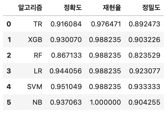
result_df = pd.DataFrame({
'알고리즘' : ['TR', 'XGB', 'RF', 'LR', 'SVM', 'NB'],
'정확도' : [acc_score1, acc_score2, acc_score3, acc_score4, acc_score5, acc_score6],
'재현율' : [rec_score1, rec_score2, rec_score3, rec_score4, rec_score5, rec_score6],
'정밀도' : [prc_score1, prc_score2, prc_score3, prc_score4, prc_score5, prc_score6]
}) ; result_df
막대 그래프로 위 데이터프레임 내용 시각화
1
2
3
4
5
6
7
8
9
10
11
12
13
14
15
16
17
18
19
plt.figure(figsize=(10,5))
plt.subplot(1,3,1)
plt.bar(range(len(result_df['알고리즘'].values)), result_df['정확도'].values)
plt.xticks(range(len(result_df['알고리즘'].values)), result_df['알고리즘'].values)
plt.ylabel('Accuracy_score')

plt.subplot(1,3,2)
plt.bar(range(len(result_df['알고리즘'].values)), result_df['재현율'].values)
plt.xticks(range(len(result_df['알고리즘'].values)), result_df['알고리즘'].values)
plt.ylabel('Recall_score')

plt.subplot(1,3,3)
plt.bar(range(len(result_df['알고리즘'].values)), result_df['정밀도'].values)
plt.xticks(range(len(result_df['알고리즘'].values)), result_df['알고리즘'].values)
plt.ylabel('Precision_score')

plt.suptitle('Models Score')
plt.tight_layout()
plt.show()
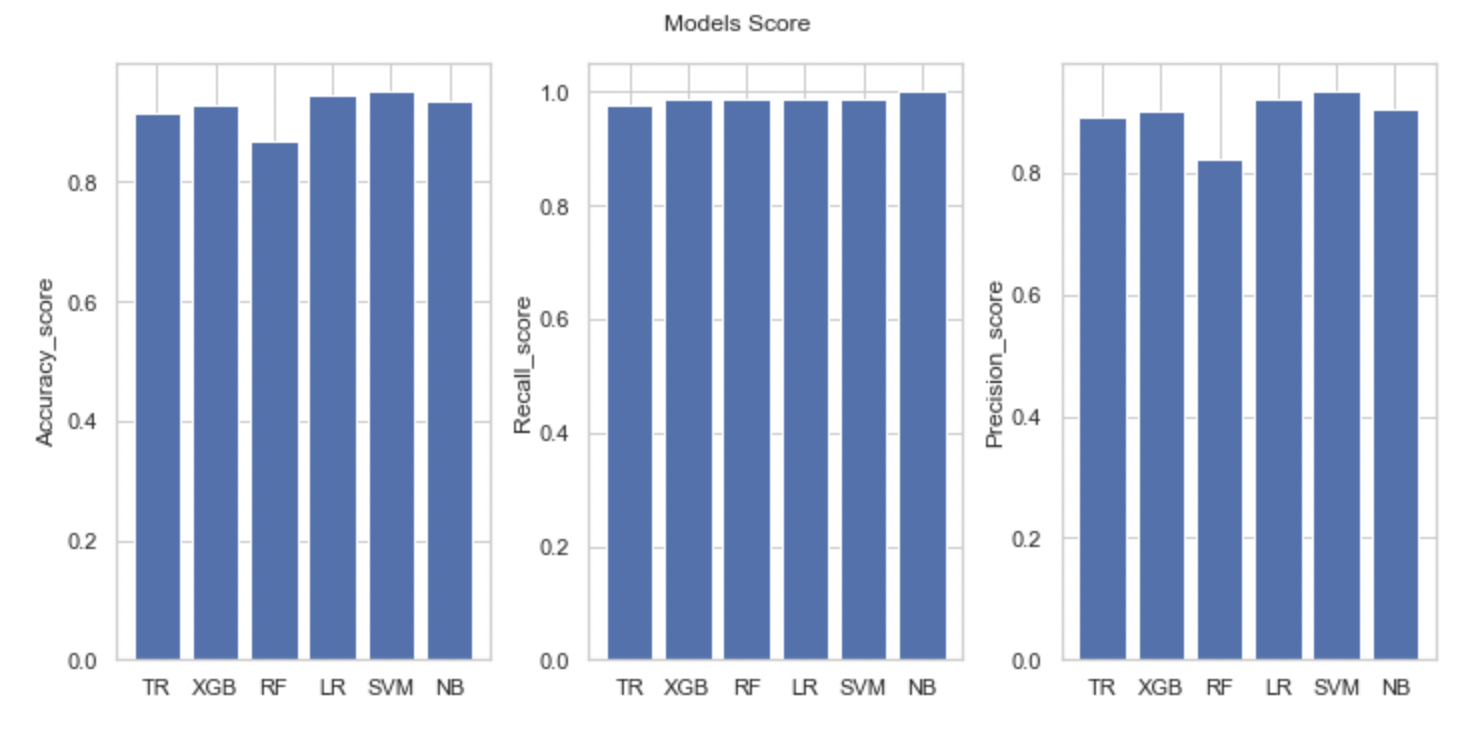
이 경우엔 대체로 서포트벡터 머신 모형이 가장 높은 성능 기록했다.