
모델 앙상블(ensemble)
정의
여러 모델 조합해서, 데이터 분류하는 알고리즘
효과
- 개별 모형보다 과적합 잘 억제할 수 있다.
- 개별 모형 성능 떨어져도, 여러 개 묶어놓으면 성능 더 향상된다.
종류
취합(aggregation)
- 다수결 투표(hard, soft voting)
- 배깅(bagging; boostrap aggregation)
- 랜덤포레스트(배깅의 한 종류)
부스팅(boosting)
- 에이다부스트(adaboost)
- 그레디언트부스트(gradient boost)
1. 취합(aggregation)
다수결 투표
- hard voting
- soft voting
- 모델 집단에 여러 종류 모델 포함할 수 있다.
Hard Voting
정의
단순 다수결 투표.
모델 집단에서 최다득점한 클래스로, 데이터 분류한다.
예컨대 모델 집단에 5개 모델이 있고, 데이터포인트 1개에 대한 각 모델 분류결과가 $(0:2)$, $(1:3)$ 이라고 하자. 단순 다수결 방식에 의하면 이 데이터포인트는 1로 분류된다.
구현
파이썬 사이킷런 라이브러리 사용해서 hard voting 방식 모델 앙상블을 구현하고, 개별 모델과 성능 비교했다.
그 후 새 데이터셋에 대한 예측 결과 시각화해서, 각 모델 별 예측 결과 비교했다.
1
2
3
4
5
6
7
8
9
10
# 모델 학습하고 성능평가할 데이터셋 구축
%matplotlib inline

from sklearn.datasets import make_gaussian_quantiles

x1, y1 = make_gaussian_quantiles(cov=2, n_samples=200, n_features=2, n_classes=2, random_state=0)
x2, y2 = make_gaussian_quantiles(mean=(3,3), cov=1.5, n_samples=200, n_features=2, n_classes=2, random_state=0)
plt.title('sample data')
plt.scatter(x1[:,0], x1[:,1]) ; plt.scatter(x2[:,0], x2[:,1], c='b')
plt.show()
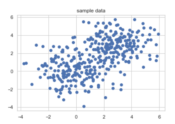
클래스 2개 (0과 1), 특성값 2개, 총 400개 데이터포인트(레코드)로 구성된 데이터셋이다.
1
2
3
4
5
6
7
# 두 파트로 구성된 데이터셋을 하나로 합친다; X, y
X = np.concatenate([x1, x2], axis=0)
y = np.concatenate([y1, y2], axis=0)

# 모델 훈련 데이터와 검증 데이터로 분리한다.
from sklearn.model_selection import train_test_split
x_train, x_test, y_train, y_test = train_test_split(X, y, test_size=0.25)
두 파트로 구성된 데이터셋을 하나로 합치고, 훈련셋과 검증셋 두 파트로 분리했다.
1
2
3
4
5
6
7
8
9
10
11
12
13
14
15
16
17
18
19
20
# 모델 앙상블 구축
from sklearn.linear_model import LogisticRegression
from sklearn.naive_bayes import GaussianNB
from sklearn.discriminant_analysis import QuadraticDiscriminantAnalysis
from sklearn.ensemble import VotingClassifier
from sklearn.metrics import accuracy_score

model1 = LogisticRegression(random_state=1)
model2 = GaussianNB()
model3 = QuadraticDiscriminantAnalysis()

# 모델 앙상블
model_ensemble = VotingClassifier(estimators=[('lr', model1), ('gnb', model2), ('qda', model3)], voting='hard')

result1 = accuracy_score(y_test, model1.fit(x_train, y_train).predict(x_test))
result2 = accuracy_score(y_test, model2.fit(x_train, y_train).predict(x_test))
result3 = accuracy_score(y_test, model3.fit(x_train, y_train).predict(x_test))
result4 = accuracy_score(y_test, model_ensemble.fit(x_train, y_train).predict(x_test))

print(f'로지스틱회귀 검증셋 정확도: {result1}') ; print(f'가우시안 나이브베이즈 검증셋 정확도 : {result2}') ; print(f'QDA 모형 검증셋 정확도: {result3}')
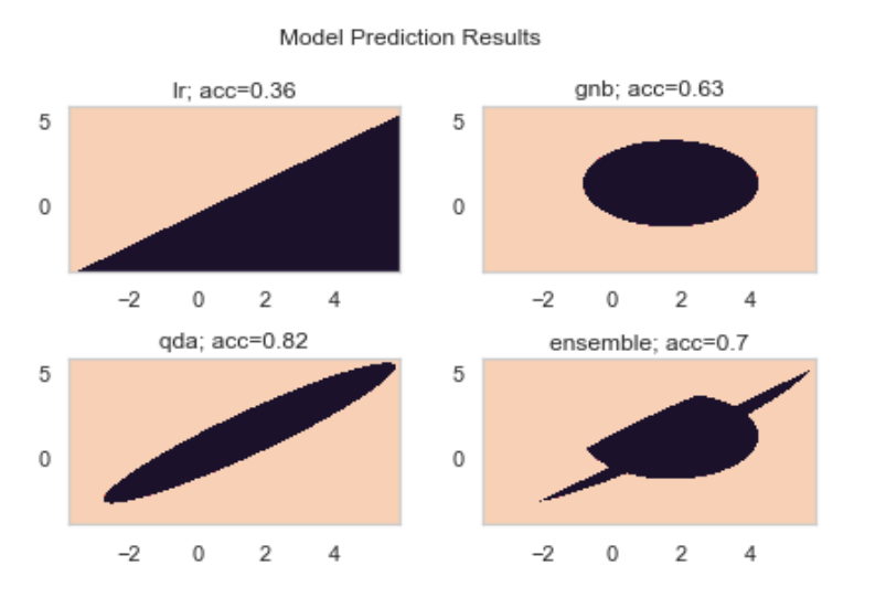
로지스틱 회귀, GNB, QDA, 그리고 셋을 조합한 모델 앙상블을 구축했다. 모델 앙상블의 voting 방식은 hard voting을 적용했다. 따라서 모델 앙상블 구성하는 세 모델의 분류 결과를 가지고 단순 다수결 투표 한 게 최종 결과가 될 것이다.
개별 모델들과 모델 앙상블의 정확도 출력했다.
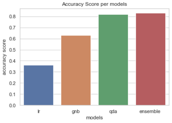
로지스틱회귀 검증셋 정확도: 0.36
가우시안 나이브베이즈 검증셋 정확도 : 0.63
QDA 모형 검증셋 정확도: 0.82
모델 앙상블 검증셋 정확도: 0.7
아래 막대그래프는 위 모델 별 정확도를 시각화 한 것이다.
1
2
3
4
5
6
7
import seaborn as sns
sns.barplot([1,2,3,4], [result1, result2, result3, result4])
plt.xticks([0,1,2,3], ['lr', 'gnb', 'qda', 'ensemble'])
plt.xlabel('models')
plt.ylabel('accuracy score')
plt.title('Accuracy Score per models')
plt.show()
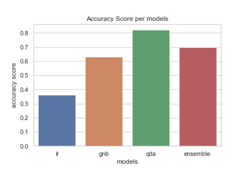
이 데이터에 대해서는 QDA 가 가장 성능이 높게 나왔다.
하지만 앙상블도 LR, GNB보다 높은 성능을 보였고, QDA와도 그렇게까지 큰 성능차 나지 않았다.
이제부터 새 데이터셋에 대해 예측하고, 예측 결과를 시각화 할 것이다.
1
2
3
4
5
6
7
8
9
# 모델 예측 결과 시각화 - 2
x1min, x1max = X[:,0].min(), X[:,0].max()
x2min, x2max = X[:,1].min(), X[:,1].max()

# 예측할 샘플 데이터셋
xx1, xx2 = np.meshgrid(np.arange(x1min, x1max, 0.01), np.arange(x2min, x2max, 0.01))
X2 = np.c_[xx1.ravel() , xx2.ravel()]

plt.scatter(xx1, xx2)
위 데이터셋은 다음과 같이 생겼다.
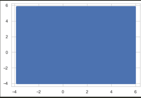
무수히 많은 점들이 직사각형을 이루고 있다. 점들 간 간격을 늘리면 아래와 같아진다.
1
2
xx1, xx2 = np.meshgrid(np.arange(x1min, x1max, 1), np.arange(x2min, x2max, 1))
plt.scatter(xx1, xx2)
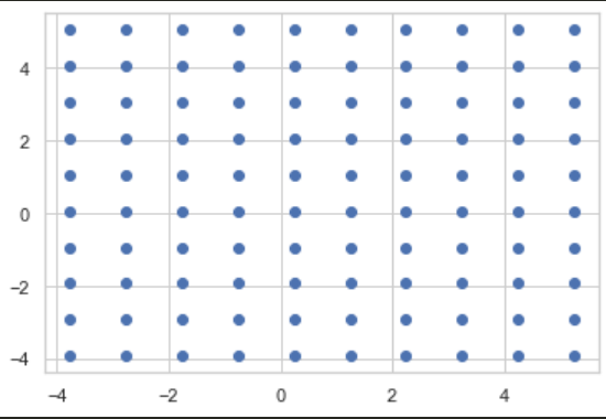
이제 앞에서 훈련한 모델들에게 위 데이터셋을 예측하도록 시켰다.
1
2
3
4
5
6
7
8
9
10
11
12
13
14
15
16
17
18
19
20
21
22
23
24
25
26
27
28
29
30
31
# 개별모델3, 앙상블1 훈련
model1 = model1.fit(x_train, y_train)
model2 = model2.fit(x_train, y_train)
model3 = model3.fit(x_train, y_train)
ensemble = model_ensemble.fit(x_train, y_train)

# 샘플 데이터셋 X2 예측
Y1 = model1.predict(X2).reshape(xx1.shape)
Y2 = model2.predict(X2).reshape(xx1.shape)
Y3 = model3.predict(X2).reshape(xx1.shape)
Y4 = ensemble.predict(X2).reshape(xx1.shape)

plt.subplot(2,2,1)
plt.contourf(xx1, xx2, Y1)
plt.title(f'lr; acc={result1}')

plt.subplot(2,2,2)
plt.contourf(xx1, xx2, Y2)
plt.title(f'gnb; acc={result2}')

plt.subplot(2,2,3)
plt.contourf(xx1, xx2, Y3)
plt.title(f'qda; acc={result3}')

plt.subplot(2,2,4)
plt.contourf(xx1, xx2, Y4)
plt.title(f'ensemble; acc={result4}')

plt.suptitle('Model Prediction Results')
plt.tight_layout()
plt.show()
실제 데이터셋 0과 1 분포
1
2
3
4
5
6
7
idx0 = np.where(y == 0)
idx1 = np.where(y == 1)

plt.title('sample data')
plt.scatter(X[idx0,0], X[idx0,1], c='r', label='class:0') ; plt.scatter(X[idx1,0], X[idx1,1], c='b', label='class:1')
plt.legend()
plt.show()

Soft Voting - 평균 방식
정의
각 모델, 클래스별 조건부확률 평균 비교해서. 평균값 가장 큰 클래스로 데이터포인트 분류하는 방법.
예컨대 이진분류 문제이고, 앙상블 모델 집단에 모델 1,2,3,4 가 있다고 가정하자.
1개 데이터포인트에 대해서;
모델1 조건부확률분포: $[0.3, 0.7]$
모델2 조건부확률분포: $[0.2, 0.8]$
모델3 조건부확률분포: $[0.5, 0.5]$
모델4 조건부확률분포: $[0.6, 0.4]$
라고 가정하자.
0 클래스 조건부확률 평균 $= \frac{0.3+0.2+0.5+0.6}{4} = 0.4$
1 클래스 조건부확률 평균 $= \frac{0.7+0.8+0.5+0.4}{4} = 0.6$
1 클래스 조건부확률 평균이 더 크므로, 이 데이터포인트는 클래스 1로 분류된다.
Soft Voting - 가중합 방식
정의
각 모델, 클래스별 조건부확률 가중합($\sum$ 모델 별 가중치 $\times$ 클래스 별 조건부확률) 비교해서 결과값 가장 큰 클래스로 데이터포인트 분류하는 방법.
예컨대 이진분류 문제이고, 앙상블 모델 집단에 모델 1,2,3 이 있다고 가정하자.
1개 데이터포인트에 대해서;
모델 1 조건부확률분포: $[0.3, 0.7]$, 모델 가중치 2
모델 2 조건부확률분포: $[0.2, 0.8]$, 모델 가중치 1
모델 3 조건부확률분포: $[0.6, 0.4]$, 모델 가중치 1
이라고 가정하자.
0 클래스 가중합 $= (0.3\times{2}) + (0.2\times{1}) + (0.6 \times{1}) = 1.4$
1 클래스 가중합 $= (0.7\times{2}) + (0.8\times{1}) + (0.4\times{1}) = 2.6$
$\therefore$ 1 클래스 가중합 결과가 더 크므로, 이 데이터포인트는 클래스 1로 분류된다.
Soft Voting 구현
1- soft voting 평균 방식
1
2
3
4
5
6
7
8
9
10
11
12
13
14
15
16
# soft voting 방식 - 평균 방식

model1 = LogisticRegression(random_state=1)
model2 = GaussianNB()
model3 = QuadraticDiscriminantAnalysis()

# 모델 앙상블
model_ensemble = VotingClassifier(estimators=[('lr', model1), ('gnb', model2), ('qda', model3)], voting='soft')

result1 = accuracy_score(y_test, model1.fit(x_train, y_train).predict(x_test))
result2 = accuracy_score(y_test, model2.fit(x_train, y_train).predict(x_test))
result3 = accuracy_score(y_test, model3.fit(x_train, y_train).predict(x_test))
result4 = accuracy_score(y_test, model_ensemble.fit(x_train, y_train).predict(x_test))

print(f'로지스틱회귀 검증셋 정확도: {result1}') ; print(f'가우시안 나이브베이즈 검증셋 정확도 : {result2}') ; print(f'QDA 모형 검증셋 정확도: {result3}')
print(f'모델 앙상블 검증셋 정확도: {result4}')
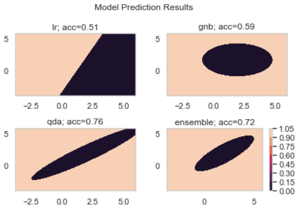
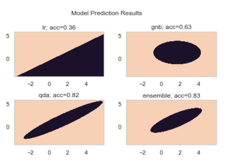
로지스틱회귀 검증셋 정확도: 0.36
가우시안 나이브베이즈 검증셋 정확도 : 0.63
QDA 모형 검증셋 정확도: 0.82
모델 앙상블 검증셋 정확도: 0.83
1
2
3
4
5
6
7
import seaborn as sns
sns.barplot([1,2,3,4], [result1, result2, result3, result4])
plt.xticks([0,1,2,3], ['lr', 'gnb', 'qda', 'ensemble'])
plt.xlabel('models')
plt.ylabel('accuracy score')
plt.title('Accuracy Score per models')
plt.show()
각 모델에 대한 새 데이터셋 예측 결과
1
2
3
4
5
6
7
8
9
10
11
12
13
14
15
16
17
18
19
20
21
22
23
24
25
26
27
28
29
30
31
32
33
34
35
36
37
38
39
40
# 모델 예측 결과 시각화 - 2
x1min, x1max = X[:,0].min(), X[:,0].max()
x2min, x2max = X[:,1].min(), X[:,1].max()

# 예측할 샘플 데이터셋
xx1, xx2 = np.meshgrid(np.arange(x1min, x1max, 0.01), np.arange(x2min, x2max, 0.01))
X2 = np.c_[xx1.ravel() , xx2.ravel()]

# 개별모델3, 앙상블1 훈련
model1 = model1.fit(x_train, y_train)
model2 = model2.fit(x_train, y_train)
model3 = model3.fit(x_train, y_train)
ensemble = model_ensemble.fit(x_train, y_train)

# 샘플 데이터셋 X2 예측
Y1 = model1.predict(X2).reshape(xx1.shape)
Y2 = model2.predict(X2).reshape(xx1.shape)
Y3 = model3.predict(X2).reshape(xx1.shape)
Y4 = ensemble.predict(X2).reshape(xx1.shape)

# 시각화
plt.subplot(2,2,1)
plt.contourf(xx1, xx2, Y1)
plt.title(f'lr; acc={result1}')

plt.subplot(2,2,2)
plt.contourf(xx1, xx2, Y2)
plt.title(f'gnb; acc={result2}')

plt.subplot(2,2,3)
plt.contourf(xx1, xx2, Y3)
plt.title(f'qda; acc={result3}')

plt.subplot(2,2,4)
plt.contourf(xx1, xx2, Y4)
plt.title(f'ensemble; acc={result4}')

plt.suptitle('Model Prediction Results')
plt.tight_layout()
plt.show()
soft voting 가중합 방식 사용하려면 모델 앙상블 객체 생성할 때, weight 파라미터에 모델 별 가중치 배열을 넣어주면 된다.
Voting 연습문제
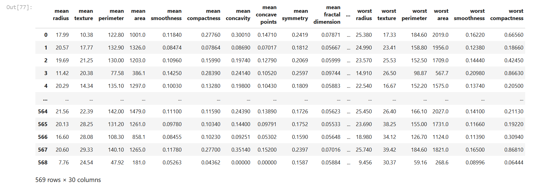
breast_cancer 데이터셋에 모델 앙상블 적용해서 분류하기.
1
2
3
4
5
6
7
8
9
from sklearn.datasets import load_breast_cancer

data = load_breast_cancer()

x = data.data
y = data.target
feature_names = data.feature_names

df = pd.DataFrame(x, columns=feature_names ) ; df
1
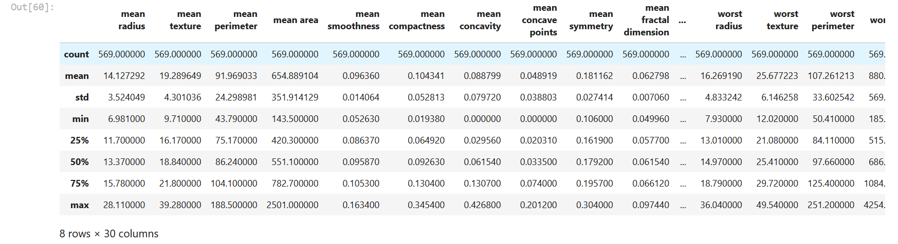
df.describe()
1
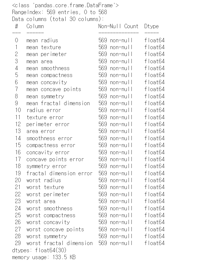
df.info()
1
df.isnull().sum().values
array([0, 0, 0, 0, 0, 0, 0, 0, 0, 0, 0, 0, 0, 0, 0, 0, 0, 0, 0, 0, 0, 0, 0, 0, 0, 0, 0, 0, 0, 0], dtype=int64)
1
2
3
4
5
6
7
8
9
10
11
12
13
14
15
16
17
18
19
20
21
22
23
24
25
26
27
28
from sklearn.model_selection import train_test_split
x_train, x_test, y_train, y_test = train_test_split(x, y, test_size=0.25, random_state=0)
from sklearn.model_selection import cross_val_score
model1 = LogisticRegression(random_state=1)
model2 = QuadraticDiscriminantAnalysis()
model3 = GaussianNB()
ensemble = VotingClassifier([('lr', model1), ('qda', model2), ('gnb', model3)], voting='hard')
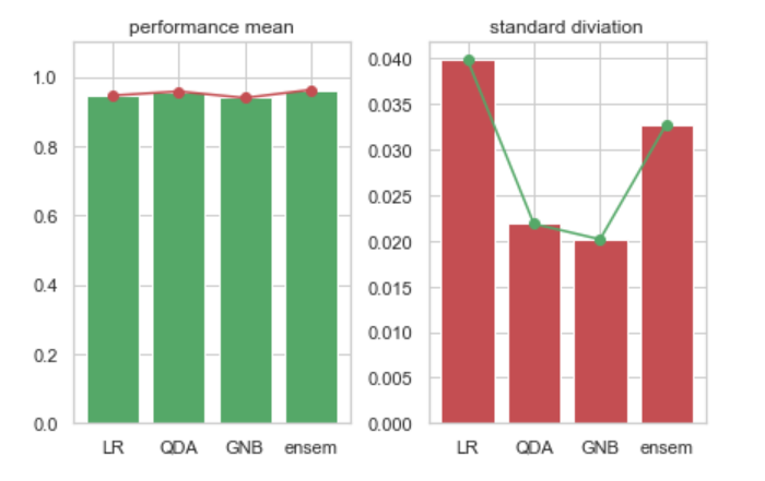
result_train = [(cross_val_score(model, x_train, y_train, scoring='accuracy', cv=5).mean(), np.std(cross_val_score(model, x_train, y_train, scoring='accuracy'))
# 시각화
plt.subplot(1,2,1)
plt.bar(np.arange(4), [r[0] for r in result_train], color='g')
plt.plot(np.arange(4), [r[0] for r in result_train ], 'ro-')
plt.ylim([0, 1.1])
plt.title('performance mean')
plt.xticks(np.arange(4), ['LR', 'QDA', 'GNB', 'ensem'])
plt.subplot(1,2,2)
plt.bar(np.arange(4), [r[1] for r in result_train], color='r')
plt.plot(np.arange(4), [r[1] for r in result_train], 'go-')
plt.xticks(np.arange(4), ['LR', 'QDA', 'GNB', 'ensem'])
plt.title('standard diviation')
plt.tight_layout()
plt.show()
1
2
3
4
5
6
7
8
result_test = [model.fit(x_train, y_train).predict(x_test) for model in (model1, model2, model3, ensemble)]
from sklearn.metrics import accuracy_score

test_acc = [accuracy_score(r, y_test) for r in result_test]
plt.plot(np.arange(4), test_acc, 'ro-')
plt.xticks(np.arange(4), ['lr', 'qda', 'gnb', 'ensem'])
plt.title('accuracy_score for test data')
plt.show()
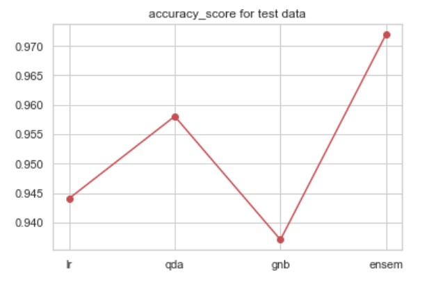
$\therefore$ 앙상블 모델이 개별모델보다 더 높은 성능 기록했다.
배깅(Bagging)
Boostrap Aggregation
정의
부스트랩으로 생성된 여러 데이터셋으로 여러 약한 분류기(weak learner) 훈련시키고, 훈련된 약분류기들의 분류 결과를 다수결 투표 하는 분류 알고리즘.
- 모델 집합으로, 같은 종류 모형 여러 개 쓴다.
부스트랩(Boostrap)
정의: 원본 데이터셋 특성변수들 랜덤으로 선발해서, 데이터셋 여러 개 만들기
예시
- 랜덤포레스트(Random Forest)
구현
의사결정나무를 약 분류기로 사용한, 배깅 모형
1
2
3
4
5
6
7
8
9
10
11
12
13
14
15
16
17
18
19
20
from sklearn.ensemble import BaggingClassifier
from sklearn.datasets import load_iris
from sklearn.tree import DecisionTreeClassifier

iris = load_iris()
x, y = iris.data[:, [0,2]], iris.target

x_train, x_test, y_train, y_test = train_test_split(x, y, random_state=0, test_size=0.25)

# 단일 의사결정나무 분류기
model1 = DecisionTreeClassifier(max_depth=10, random_state=0).fit(x_train, y_train)

# 배깅 모형 분류기; 100개 단일 의사결정나무 모형으로 구성.
model2 = BaggingClassifier(DecisionTreeClassifier(max_depth=2), n_estimators=100, random_state=0).fit(x_train, y_train)

# 단일 의사결정나무 분류기 예측
print(f'단일 의사결정나무 분류기 예측 정확도: {accuracy_score(model1.predict(x_test), y_test)}')

# 배깅 모형 분류기 예측
print(f'배깅 모형 분류기 예측 정확도: {accuracy_score(model2.predict(x_test), y_test)}')
단일 의사결정나무 분류기 예측 정확도: 0.8947368421052632
배깅 모형 분류기 예측 정확도: 0.8947368421052632
$\Rightarrow$ 단일 모형보다 훨씬 깊이 얕은 의사결정나무 100개 엮었더니, 단일모형과 같은 예측 정확도 달성했다.
연습문제
breast cancer 데이터셋에 배깅 모형 적용해서 분류문제 해결하기
1
2
3
4
5
6
7
8
9
10
11
12
13
14
15
16
17
18
19
20
21
## 연습문제 2

from sklearn.datasets import load_breast_cancer

bc = load_breast_cancer()
x = bc.data
y = bc.target

x_train, x_test, y_train, y_test = train_test_split(x, y, random_state=0, test_size=0.3)

from sklearn.svm import SVC
from sklearn.ensemble import BaggingClassifier

model = BaggingClassifier(SVC(), n_estimators=10, random_state=0).fit(x_train, y_train)
model2 = SVC().fit(x_train, y_train)

model_result = cross_val_score(model, x_test, y_test, scoring='accuracy', cv=5).mean()
model2_result = cross_val_score(model2, x_test, y_test, scoring='accuracy', cv=5).mean()

print(f'배깅모델 교차검증 정확도: {model_result}')
print(f'단일모델 교차검증 정확도: {model2_result}')
배깅모델 교차검증 정확도: 0.9302521008403362
단일모델 교차검증 정확도: 0.9184873949579831
$\Rightarrow$ 배깅모형의 교차검증 정확도가 단일모델보다 약간 더 높았다.
랜덤포레스트(Random Forest)
정의
약 분류기로 의사결정나무를 사용한, 배깅 모델.
각 하위 의사결정나무에서 노드 분리 시, 데이터셋 독립변수 차원을 랜덤하게 감소시킨 뒤, 남은 독립변수들 중에서 분류규칙을 결정한다.
각 하위 의사결정나무에서, 노드 분리 할 때 마다 랜덤하게 분류규칙 정하는 경우, Extremely Randomized Trees 모형 이라고 별칭한다.
구현
1
2
3
4
5
6
7
8
9
10
11
12
13
14
15
16
17
18
19
20
21
# 랜덤포레스트 - 배깅모델의 한 종류
from sklearn.datasets import load_iris
from sklearn.tree import DecisionTreeClassifier
from sklearn.ensemble import RandomForestClassifier

# iris 데이터셋 로드
iris = load_iris()

x, y = iris.data[:, [0,2]], iris.target

# 훈련, 테스트용 데이터셋으로 분리
x_train, x_test, y_train, y_test = train_test_split(x, y, random_state=0, test_size=0.25)

# 단일 의사결정나무 분류기
model1 = DecisionTreeClassifier(max_depth=10, random_state=10).fit(x_train, y_train)

# 랜덤포레스트 분류기; 100개 의사결정나무로 구성
model2 = RandomForestClassifier(max_depth=2, n_estimators=100, random_state=0).fit(x_train, y_train)

print(f'단일 의사결정나무 정확도: {accuracy_score(y_test, model1.predict(x_test))}')
print(f'랜덤포레스트 정확도: {accuracy_score(y_test, model2.predict(x_test))}')
단일 의사결정나무 정확도: 0.8947368421052632
랜덤포레스트 정확도: 0.8947368421052632
랜덤포레스트; 특성변수 별 중요도 계산
$a_{i} = $ 하위 의사결정나무(약 분류기) $i$ 내 특성변수 별 정보획득량 평균
$n = $ 랜덤포레스트 내부 의사결정나무 갯수
특성변수 별 중요도 $= \frac{1}{n}\sum{a_{i}}$
예제
1
2
3
4
5
6
7
8
9
10
11
12
13
14
15
16
17
18
19
20
21
22
23
24
25
26
27
28
29
30
31
32
33
# 분류모델 테스트용; 조건에 맞는 가상데이터 생성
from sklearn.datasets import make_classification
from sklearn.ensemble import ExtraTreesClassifier

# 모델 테스트용 가상데이터
x, y = make_classification(n_samples=1000, n_features=10, n_informative=3, n_redundant=0, n_classes=2, random_state=0, shuffle=False)

# 의사결정나무 250개로 구성된 extreme 랜덤포레스트
forest = ExtraTreesClassifier(n_estimators=250, random_state=0)
forest.fit(x, y)

# 랜덤포레스트 알고리즘 내에서, 각 특성변수 별 중요도
importances = forest.feature_importances_

# 일반 랜덤포레스트에 대해서도 정보획득량 평균 구할 수 있다.
rf = RandomForestClassifier(max_depth=2, n_estimators=100, random_state=0).fit(x, y)
rf.feature_importances_

# 여러 하위 의사결정나무에 걸친, 특성변수 중요도 표준편차
std = np.std([tree.feature_importances_ for tree in forest.estimators_], axis=0)

# 내림차순 정렬했을 때 요소들 리스트 순서
indicies = np.argsort(importances)[::-1]

# 시각화
plt.bar(range(10), importances[indicies], color= 'r', yerr=std[indicies], align='center')
plt.xticks(range(x.shape[1]), indicies)

plt.xlim([-1, x.shape[1]])
plt.title('The importance of feature variables')
plt.xlabel('n_feature variables')
plt.ylabel('importance')
plt.show()
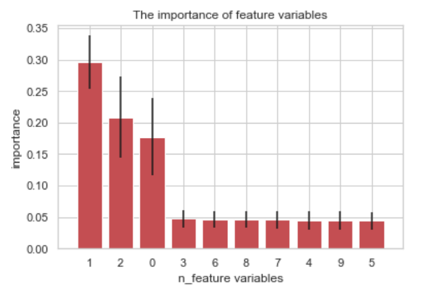
0~9번 특성변수 별 중요도 및 표준편차
예제 2; 각 이미지 분류하는 데 결정적 기여하는, 중요한 픽셀만 골라내기
1
2
3
4
5
6
7
8
9
10
11
# 올리베티 얼굴사진 데이터에 랜덤포레스트 적용하기

from sklearn.datasets import fetch_olivetti_faces
from sklearn.ensemble import ExtraTreesClassifier

data = fetch_olivetti_faces()
x = data.data ; y = data.target

x_train, x_test, y_train, y_test = train_test_split(x, y, random_state=0, test_size=0.25)

r_forest = RandomForestClassifier(random_state=2, n_estimators=250).fit(x_train, y_train)
픽셀 별 중요도 시각화
1
2
3
4
5
6
7
8
9
# 각 픽셀 별 정보획득량 평균(픽셀 별 중요도)
fi = r_forest.feature_importances_

fi_2 = fi.reshape(data.images[0].shape)

plt.imshow(fi_2, cmap=plt.cm.bone_r)
plt.axis('off')
plt.title('Each pixcel importance')
plt.show()
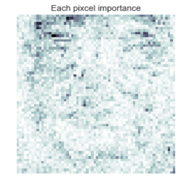
중요 픽셀일 수록 정보획득량 평균이 높아 진하게 표시,
덜 중요한 픽셀 일 수록 정보획득량 평균이 낮아 연하게 표시된다.
1
accuracy_score(y_test, r_forest.predict(x_test))
0.97
연습문제
breast cancer 데이터에 랜덤포레스트 적용해서 데이터포인트 분류하기
1
2
3
4
5
6
7
8
9
10
11
12
13
14
15
16
17
18
# 연습문제 3
from sklearn.datasets import load_breast_cancer
from sklearn.model_selection import train_test_split
from sklearn.ensemble import ExtraTreesClassifier
from sklearn.model_selection import cross_val_score

data = load_breast_cancer()
x = data.data
y = data.target

x_train, x_test, y_train, y_test = train_test_split(x, y, random_state=0, test_size=0.3)

# extreme random forest 모델
tree = ExtraTreesClassifier(random_state=0, n_estimators=250)
tree.fit(x_train, y_train)

print(f'훈련용 데이터에 대해 교차검증 평균성능 : {cross_val_score(tree, x_train, y_train, scoring="accuracy", cv=5).mean()}')
print(f'테스트용 데이터에 대해 교차검증 평균성능: {cross_val_score(tree, x_test, y_test, scoring="accuracy",cv=5).mean()}')
훈련용 데이터에 대해 교차검증 평균성능 : 0.9623734177215191
테스트용 데이터에 대해 교차검증 평균성능: 0.9532773109243697
1
2
3
4
5
6
7
importances = tree.feature_importances_
indice = np.argsort(importances)
%matplotlib inline
plt.barh(range(len(importances)), importances[indice])
plt.yticks(range(len(importances)), data.feature_names[indice])
plt.tight_layout()
plt.show()
